Session 08: DA with SQL | JOINs

SQL

Normalization

JOINs

Normalization

Relational databases do not start with JOINs.
They start with structure.

Normalization explains why data is split, and JOINs explain how it is recombined.

If this logic is not clear, JOINs feel like a technical burden instead of a logical necessity.

Problem

The Core Problem: Redundancy and Anomalies

Imagine storing everything in a single table.

We are saying Unnormalized Design:

order_id	customer_name	city	product	price	quantity
1	Anna	Yerevan	Phone	500	1
2	Anna	Yerevan	Case	20	2
3	Arman	Gyumri	Phone	500	1

Customer data is duplicated
Product prices are duplicated
Updates are risky
Deletes may remove important information
Inserts may require fake or incomplete values

This structure is fragile and error-prone.

First Normal Form (1NF)

A table is in First Normal Form (1NF) if:

Each column contains atomic values
There are no repeating groups
Each row is uniquely identifiable

Important

The table above already satisfies 1NF, but it is still poorly designed because multiple entities are mixed together.

erDiagram
    ORDERS {
        int order_id
        string customer_name
        string city
        string product
        float price
        int quantity
    }

Second Normal Form (2NF)

A table is in Second Normal Form (2NF) if:

It is already in 1NF
No non-key attribute depends on part of a composite key

To understand this, we must first identify the logical key of the original table.

In the unnormalized table, the logical key is: (order_id, product)

because:

one order can contain multiple products
quantity is defined per product per order

Problem

Look at the dependencies:

customer_name, city depend only on order_id
price depends only on product
quantity depends on (order_id, product)

This means we have partial dependencies.

Some columns depend on only part of the key, not the whole key.

\[\downarrow\]

This violates 2NF.

flowchart LR
    K[(order_id, product)]
    K --> Q[quantity]
    order_id --> C[customer_name, city]
    product --> P[price]

Decomposition to 2NF

To fix this, we separate data so that each table describes exactly one relationship.

Customers

customer_id	customer_name	city

Meaning:

customer attributes depend only on customer_id

Products

product_id	product	price

Meaning:

product attributes depend only on product_id

Orders

order_id	customer_id

Meaning:

this table describes who placed the order
customer_id depends entirely on order_id

There is no composite key here, so partial dependency is impossible.

Order Items

order_id	product_id	quantity

Meaning:

this table describes what was ordered
the key is (order_id, product_id)
quantity depends on the entire key, not just one part

erDiagram
    CUSTOMERS {
        int customer_id PK
        string customer_name
        string city
    }

    PRODUCTS {
        int product_id PK
        string product
        float price
    }

    ORDERS {
        int order_id PK
        int customer_id FK
    }

    ORDER_ITEMS {
        int order_id FK
        int product_id FK
        int quantity
    }

    CUSTOMERS ||--o{ ORDERS : places
    ORDERS ||--o{ ORDER_ITEMS : contains
    PRODUCTS ||--o{ ORDER_ITEMS : included_in

Why This Satisfies 2NF

After decomposition:

Customer attributes depend only on customers:
- customer_name
- city
Product attributes depend only on products
- product_name
- price
Order attributes depend only on orders
- order_id
- customer_id
Quantity depends on both order and** product**
- order_id
- product_id
- quantity

As a result:

There are no partial dependencies left.
Each non-key attribute now depends on the entire key of its table.

\[\downarrow\]

This is exactly what Second Normal Form requires.

Third Normal Form (3NF)

After reaching Second Normal Form (2NF), we removed partial dependencies.
However, another type of problem can still exist: transitive dependencies.

A table is in Third Normal Form (3NF) if:

It is already in 2NF
No non-key attribute depends on another non-key attribute

In other words:

Every non-key attribute must depend only on the primary key and nothing else.

Transitive Dependency

A transitive dependency occurs when:

A non-key attribute depends on another non-key attribute
Instead of depending directly on the primary key

Formally:

flowchart LR
    customer_id --> city
    city --> country
    customer_id --> country

This is a transitive dependency.

Consider the Customers table after 2NF:

customer_id	customer_name	city	country

Let’s analyze the dependencies:

customer_id → city
city → country

\[\downarrow\]

customer_id → country indirectly

So country does not depend directly on customer_id.
It depends on city.

This violates Third Normal Form.

Problems

This structure creates anomalies:

If a city changes its country name, multiple rows must be updated
If the last customer from a city is deleted, the city–country relationship is lost
If a new city is added, a customer must exist first

These are update, delete, and insert anomalies caused by transitive dependency.

Decomposition to 3NF

To remove the transitive dependency, we split the table based on real-world entities.

Cities

city_id	city	country_id

Meaning:

city attributes depend only on city_id
the relationship between city and country is stored once

Countries

country_id	country

country attributes depend only on country_id

Customers

customer_id	customer_name	city_id

customer attributes depend only on customer_id

city information is referenced, not duplicated

erDiagram
    CUSTOMERS {
        int customer_id PK
        string customer_name
        int city_id FK
    }

    CITIES {
        int city_id PK
        string city
        int country_id FK
    }

    COUNTRIES {
        int country_id PK
        string country
    }

    CUSTOMERS ||--|| CITIES : lives_in
    CITIES ||--|| COUNTRIES : belongs_to

Why This Satisfies 3NF

After decomposition:

customer_name depends only on customer_id
city_id depends only on customer_id
country depends only on country_id
There are no indirect dependencies

Each table now represents one concept and one level of dependency.

Normalization Summary

First Normal Form removing duplicate rows
Second Normal Form removes partial dependencies.
Third Normal Form removes transitive dependencies.

At this point:

Data redundancy is minimized
Anomalies are eliminated
Relationships are explicit

flowchart TB
    A[Unnormalized] --> B[1NF<br/>Atomic Values]
    B --> C[2NF<br/>No Partial Dependencies]
    C --> D[3NF<br/>No Transitive Dependencies]

After 3NF…

3NF is commonly considered sufficient in practice for many transactional systems.

Boyce-Codd Normal Form (BCNF): BCNF is a stricter refinement of 3NF. A table is in BCNF if:
- For every functional dependency (X → Y), X must be a superkey (a unique identifier for the table).
- This eliminates certain anomalies that can still exist in 3NF designs.
Fourth Normal Form (4NF): Removes multi-valued dependencies (if the table is already in BCNF).
Fifth Normal Form (5NF): Eliminates join dependencies beyond 4NF.
Sixth Normal Form (6NF) and others exist mostly for theoretical completeness.

For more information you can visit here

New Analytical Schema

This schema is intentionally designed to support:

INNER / LEFT / RIGHT / FULL OUTER joins
SELF joins
SPATIAL joins
Window functions
Subqueries
CTEs

Creating a schema and tables
Populate data using CSV-based loading

Tip

Here you may find the complete solution.

In case of failure you can use below scripts:

Windows Users:
reset-db-full.ps1 completely re-runs the Docker containers and removes old containers.
reset-db.ps1 re-runs the Postgres DB while keeping pgAdmin data.
MacOS Users:
reset-db-full.sh completely re-runs the Docker containers and removes old containers.
reset-db.sh re-runs the Postgres DB while keeping pgAdmin data.

Open the terminal/PowerShell in vscode and type:

Windows Users:
- powershell -ExecutionPolicy Bypass -File reset-db.ps1
- powershell -ExecutionPolicy Bypass -File reset-db-full.ps1
MacOS Users:
- ./reset-db.sh
- ./reset-db-full.sh

Docker Update

As usual, we are starting by running our Docker containers:

the database
pgadmin (viewer)

Step 1: Stop and clean existing containers

We first stop the containers and remove volumes (-v ensures that old database data is removed).

docker compose down -v

Step 2: Update the Docker image

In docker-compose.yaml, update the database service:

Before
```
image: postgres:17
```
After
```
image: postgis/postgis:17-3.4
```
Add also a new volume
```
- ./data/analytics_schema:/data:ro
```

This image includes:

PostgreSQL 17
PostGIS 3.4
All required spatial libraries

Step 3: Remove persisted data folders

To ensure a clean initialization, delete the following folders if they exist:

postgres_data/
pgadmin_data/

These folders store old volumes and may conflict with the new image.

Step 4: Start containers again

First start normally and verify everything works:

docker compose up

Once confirmed, stop and restart in detached mode:

docker compose up -d

Add PostGIS Extension

Once the PostGIS-enabled container is running, we enable the extension inside the database.

CREATE EXTENSION IF NOT EXISTS postgis;

To verify that PostGIS is installed correctly:

SELECT PostGIS_Version();

The above code should provide a table with postgis_version: 3.4 USE_GEOS=1 USE_PROJ=1 USE_STATS=1

If this returns a version string, PostGIS is ready.

Creating New Schema

We do not use the default public schema for analytics.
Instead, we create a dedicated schema called analytics.

If you right-click on the schemas

CREATE SCHEMA IF NOT EXISTS analytics;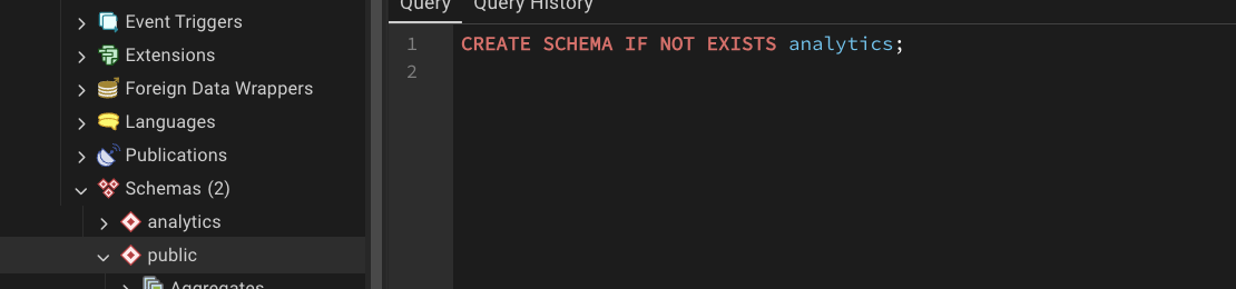

SET search_path TO analytics

PostgreSQL databases can contain multiple schemas.
When you write:

SELECT * FROM customers;

PostgreSQL must decide which schema to search for the customers table.

By default, it searches the public schema.

By running: SET search_path TO analytics; we tell PostgreSQL:

“Look in the analytics schema first when resolving table names.”

SELECT 
  *
FROM orders o
JOIN customers c ON o.customer_id = c.customer_id;

instead of:

SELECT 
  *
FROM analytics.orders o
JOIN analytics.customers c ON o.customer_id = c.customer_id;

Sync with GitHub

Remember to push the changes into GitHub:

git add docker-compose.yml
git commit -m "adding postgis extension"
git push

Creating Geographical Tables

Now we define the analytical data model that will be used throughout this module.

The schema follows a normalized (3NF) design with a clear geographic hierarchy:

Country → Region → City → Customer

You can check the newly created analytics schema, and refresh it after each new table creation.

Countries

This table represents sovereign countries and serves as the top-level geographic entity.

CREATE TABLE analytics.countries (
    country_id   INT PRIMARY KEY,
    country_name TEXT NOT NULL
);

Regions

CREATE TABLE analytics.regions (
    region_id   INT PRIMARY KEY,
    region_name TEXT NOT NULL,
    country_id  INT NOT NULL REFERENCES analytics.countries(country_id)
);

Cities

CREATE TABLE analytics.cities (
    city_id   INT PRIMARY KEY,
    city_name TEXT NOT NULL,
    region_id INT NOT NULL REFERENCES analytics.regions(region_id)
);

Creating Non Geographical Tables

Customers

CREATE TABLE analytics.customers (
    customer_id INT PRIMARY KEY,
    first_name  TEXT NOT NULL,
    last_name   TEXT NOT NULL,
    age         INT CHECK (age BETWEEN 16 AND 100),
    email       TEXT UNIQUE,
    city_id     INT REFERENCES analytics.cities(city_id),
    signup_date DATE NOT NULL
);

Products

CREATE TABLE analytics.products (
    product_id   INT PRIMARY KEY,
    product_name TEXT NOT NULL,
    category     TEXT NOT NULL,
    price        NUMERIC(10,2) NOT NULL
);

Orders

CREATE TABLE analytics.orders (
    order_id    INT PRIMARY KEY,
    customer_id INT REFERENCES analytics.customers(customer_id),
    order_date  DATE NOT NULL,
    status      TEXT NOT NULL
);

Order Items

CREATE TABLE analytics.order_items (
    order_item_id INT PRIMARY KEY,
    order_id      INT NOT NULL REFERENCES analytics.orders(order_id),
    product_id    INT NOT NULL REFERENCES analytics.products(product_id),
    quantity      INT NOT NULL CHECK (quantity > 0)
);

Country Boundaries

These tables extend the relational model with geometries, enabling spatial joins.

CREATE TABLE analytics.country_boundaries (
    country_id INT PRIMARY KEY REFERENCES analytics.countries(country_id),
    geom       GEOMETRY(MultiPolygon, 4326)
);

Region Boundaries

CREATE TABLE analytics.region_boundaries (
    region_id INT PRIMARY KEY REFERENCES analytics.regions(region_id),
    geom      GEOMETRY(Polygon, 4326)
);

City Boundaries

CREATE TABLE analytics.city_boundaries (
    city_id INT PRIMARY KEY REFERENCES analytics.cities(city_id),
    geom    GEOMETRY(Polygon, 4326)
);

Customer Locations

CREATE TABLE analytics.customer_locations (
    customer_id INT PRIMARY KEY REFERENCES analytics.customers(customer_id),
    geom        GEOMETRY(Point, 4326)
);

Design Summary

At this stage, the database contains:

A fully qualified analytics schema
Normalized relational tables (3NF)
Hierarchical geographic dimensions
Fact tables for analytical workloads
Spatial tables for PostGIS joins

Check out the this repository on my side

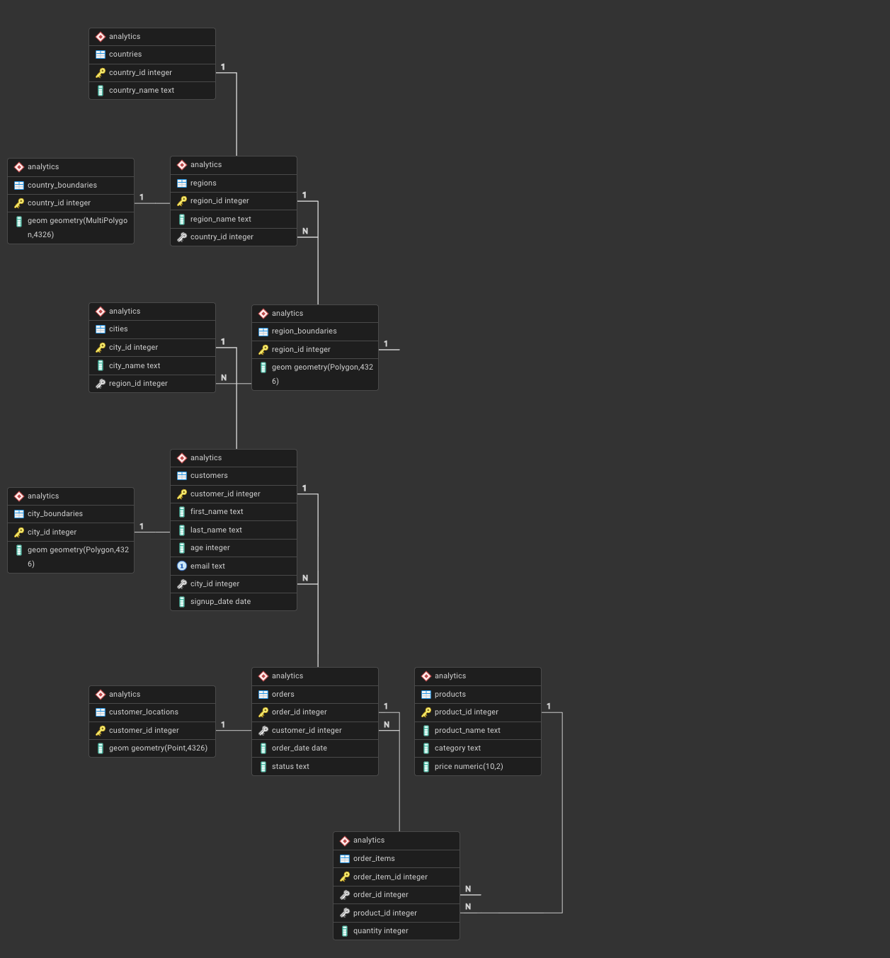
ERD

In order to generate and check the ERD, you need to:

right-click on analytics schema
select ERD
you must see below image

Important

In case you are encountering an error please do the following

function postgis_typmod_type(integer) does not exist
LINE 1: SELECT postgis_typmod_type(i) FROM
^
HINT: No function matches the given name and argument types. You might need to add explicit type casts.

DROP EXTENSION IF EXISTS postgis CASCADE;
-- SET search_path TO public;
CREATE EXTENSION postgis;
SELECT PostGIS_Version();

It should return: postgis_version: 3.4 USE_GEOS=1 USE_PROJ=1 USE_STATS=1

Sync with GitHub

Save the queries in a proper file similar to this repository and push to GitHub.

Populating the Data

In your folder now you need to have the following structure

data/
├── public_schema/
│   └── ...            # existing dummy data (unchanged)
└── analytics_schema/
    ├── countries.csv
    ├── regions.csv
    ├── cities.csv
    ├── customers.csv
    ├── products.csv
    ├── orders.csv
    ├── order_items.csv
    ├── country_boundaries.csv
    ├── region_boundaries.csv
    ├── city_boundaries.csv
    └── customer_locations.csv

Checking

try this:

SELECT pg_ls_dir('/data');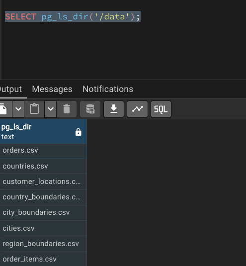

`analytics.countries`

COPY analytics.countries
FROM '/data/countries.csv'
CSV HEADER;

SELECT * FROM analytics.countries;

`analytics.regions`

COPY analytics.regions
FROM '/data/regions.csv'
CSV HEADER;

SELECT * FROM analytics.regions;

`analytics.cities`

COPY analytics.cities
FROM '/data/cities.csv'
CSV HEADER;

SELECT * FROM analytics.cities;

`analytics.customers`

COPY analytics.customers
FROM '/data/customers.csv'
CSV HEADER;

SELECT * FROM analytics.customers LIMIT 10;

`analytics.products`

COPY analytics.products
FROM '/data/products.csv'
CSV HEADER;

SELECT * FROM analytics.products;

`analytics.orders`

COPY analytics.orders
FROM '/data/orders.csv'
CSV HEADER;

SELECT * FROM analytics.orders LIMIT 10;

`analytics.order_items`

COPY analytics.order_items
FROM '/data/order_items.csv'
CSV HEADER;

SELECT * FROM analytics.order_items LIMIT 10;

Boundary Tables

Here we need to do something important transformation, by creating temporary tables

Creating `Staging` Tables

CREATE TABLE IF NOT EXISTS analytics._stg_country_boundaries (
    country_id INT,
    wkt TEXT
);


CREATE TABLE IF NOT EXISTS analytics._stg_region_boundaries (
    region_id INT,
    wkt TEXT
);

CREATE TABLE IF NOT EXISTS analytics._stg_city_boundaries (
    city_id INT,
    wkt TEXT
);

CREATE TABLE IF NOT EXISTS analytics._stg_points (
    point_id INT,
    wkt TEXT
);

COPY CSVs into staging tables

COPY analytics._stg_country_boundaries
FROM '/data/country_boundaries.csv'
CSV HEADER;

SELECT * FROM analytics._stg_country_boundaries;

COPY analytics._stg_region_boundaries
FROM '/data/region_boundaries.csv'
CSV HEADER;

SELECT * FROM analytics._stg_region_boundaries;

COPY analytics._stg_city_boundaries
FROM '/data/city_boundaries.csv'
CSV HEADER;

SELECT * FROM analytics._stg_city_boundaries;


COPY analytics._stg_points
FROM '/data/customer_locations.csv'
CSV HEADER;

SELECT * FROM analytics._stg_points;

`analytics.country_boundaries`

INSERT INTO analytics.country_boundaries (country_id, geom)
SELECT
  country_id,
  ST_GeomFromText(wkt, 4326)
FROM analytics._stg_country_boundaries;

SELECT * FROM analytics.country_boundaries;

`analytics.region_boundaries`

INSERT INTO analytics.region_boundaries (region_id, geom)
SELECT
  region_id,
  ST_GeomFromText(wkt, 4326)
FROM analytics._stg_region_boundaries;

SELECT * FROM analytics.region_boundaries;

`analytics.city_boundaries`

INSERT INTO analytics.city_boundaries (city_id, geom)
SELECT
  city_id,
  ST_GeomFromText(wkt, 4326)
FROM analytics._stg_city_boundaries;

SELECT * FROM analytics.city_boundaries;

`analytics.customer_locations`

INSERT INTO analytics.customer_locations (customer_id, geom)
SELECT
  point_id,
  ST_GeomFromText(wkt, 4326)
FROM analytics._stg_points;

SELECT * FROM analytics.customer_locations;

Geometry checks

SELECT
  COUNT(*) FILTER (WHERE ST_IsValid(geom)) AS valid_geom,
  COUNT(*) AS total
FROM analytics.country_boundaries;

SELECT
  ST_GeometryType(geom),
  COUNT(*)
FROM analytics.country_boundaries
GROUP BY 1;

Geometry Validation

SELECT
  COUNT(*) FILTER (WHERE ST_IsValid(geom)) AS valid_geometries,
  COUNT(*) AS total_geometries
FROM analytics.city_boundaries;

SELECT
  COUNT(*) FILTER (WHERE ST_SRID(geom) = 4326) AS correct_srid,
  COUNT(*) AS total_geometries
FROM analytics.city_boundaries;

Table JOINs

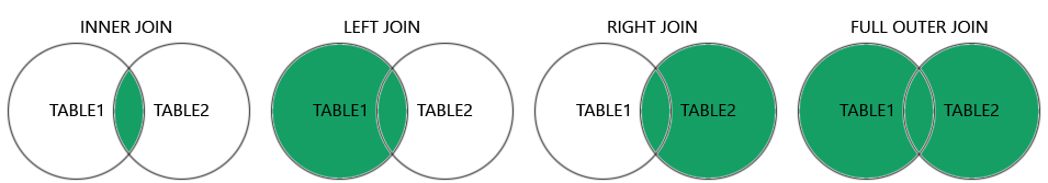
INNER JOIN | Only Matching Rows

Question: Which customers have placed orders?

Only rows where customers.customer_id = orders.customer_id are kept.

SELECT
  c.customer_id,
  c.first_name,
  o.order_id,
  o.order_date
FROM analytics.customers c
INNER JOIN analytics.orders o
  ON c.customer_id = o.customer_id;

Customers without orders are excluded
Orders without customers are excluded

LEFT JOIN | Preserve the Base Table

Question: Show all customers, even if they never ordered.

flowchart LR
  C[customers] -->|customer_id| O[orders]
  C --> R[Result]
  O --> R

All customers are preserved.
Orders are optional.

SELECT
  c.customer_id,
  c.first_name,
  o.order_id
FROM analytics.customers c
LEFT JOIN analytics.orders o
  ON c.customer_id = o.customer_id;

Customers without orders appear with NULL values
Base table = customers

LEFT JOIN + NULL FILTER | Anti-Join Pattern

Question: Which customers have never ordered?

flowchart LR
  C[customers] -->|customer_id| O[orders]
  O -. no match .-> N[NULL]

SELECT
  c.customer_id,
  c.first_name
FROM analytics.customers c
LEFT JOIN analytics.orders o
  ON c.customer_id = o.customer_id
WHERE o.order_id IS NULL;

Very common interview and analytics pattern
Identifies absence of relationships

One-to-Many JOIN | Orders to Order Items

Question: What products were sold in each order?

flowchart LR
  O[orders] -->|order_id| OI[order_items] -->|product_id| P[products]

SELECT
  o.order_id,
  p.product_name,
  oi.quantity
FROM analytics.orders o
JOIN analytics.order_items oi
  ON o.order_id = oi.order_id
JOIN analytics.products p
  ON oi.product_id = p.product_id;

One order → many order items
Rows multiply by design

Aggregation After JOIN | Controlling Row Explosion

Question: Total revenue per order.

flowchart LR
  O[orders] --> OI[order_items] --> P[products]
  P --> SUM[Sum of quantity times price]

SELECT
  o.order_id,
  SUM(oi.quantity * p.price) AS order_revenue
FROM analytics.orders o
JOIN analytics.order_items oi
  ON o.order_id = oi.order_id
JOIN analytics.products p
  ON oi.product_id = p.product_id
GROUP BY o.order_id;

Aggregation collapses multiplied rows
Critical in analytical SQL

Hierarchical JOIN | Customer Geography

Question: Where is each customer located?

flowchart LR
  CO[countries] --> R[regions] --> CI[cities] --> C[customers]

SELECT
  c.customer_id,
  ci.city_name,
  r.region_name,
  co.country_name
FROM analytics.customers c
JOIN analytics.cities ci
  ON c.city_id = ci.city_id
JOIN analytics.regions r
  ON ci.region_id = r.region_id
JOIN analytics.countries co
  ON r.country_id = co.country_id;

Dimension-style hierarchy
Common in BI models

Spatial JOIN | Geometry Meets Business Data

Question: Is a customer physically inside their declared city?

flowchart LR
  CL[customer_locations] -->|ST_Within| CB[city_boundaries]

SELECT
  c.customer_id,
  ci.city_name,
  ST_Within(cl.geom, cb.geom) AS inside_city
FROM analytics.customers c
JOIN analytics.customer_locations cl
  ON c.customer_id = cl.customer_id
JOIN analytics.cities ci
  ON c.city_id = ci.city_id
JOIN analytics.city_boundaries cb
  ON ci.city_id = cb.city_id;

Combines relational joins with spatial predicates
Typical PostGIS analytical pattern

Tip

Many-to-Many Effect | Why Row Counts Explode

flowchart LR
  O[orders] --> OI[order_items]
  OI --> P[products]

SELECT COUNT(*) AS joined_rows
FROM analytics.orders o
JOIN analytics.order_items oi
  ON o.order_id = oi.order_id;

Each order may contain multiple products
Each product may appear in many orders
Analysts must expect multiplication

Homework

Normalize this table
Answer these questions from our database:
- Q1: Who are our customers and where are they located?
- Q2: Do we have customers who have never placed an order?
- Q3: Why does joining orders to order items increase row count?
- Q4: What products were sold, to whom, and where?
- Q5: Total revenue per country.
- Q6: Are there customers without a city?
Start thinking about the final project.

Normalization

Problem

First Normal Form (1NF)

Second Normal Form (2NF)

Problem

Decomposition to 2NF

Customers

Products

Orders

Order Items

Why This Satisfies 2NF

Third Normal Form (3NF)

Transitive Dependency

Problems

Decomposition to 3NF

Cities

Countries

Customers

Why This Satisfies 3NF

Normalization Summary

New Analytical Schema

Docker Update

Step 1: Stop and clean existing containers

Step 2: Update the Docker image

Step 3: Remove persisted data folders

Step 4: Start containers again

Add PostGIS Extension

Creating New Schema

Sync with GitHub

Creating Geographical Tables

Countries

Regions

Cities

Creating Non Geographical Tables

Customers

Products

Orders

Order Items

Country Boundaries

Region Boundaries

City Boundaries

Customer Locations

Design Summary

ERD

Sync with GitHub

Populating the Data

Checking

analytics.countries

analytics.regions

analytics.cities

analytics.customers

analytics.products

analytics.orders

analytics.order_items

Boundary Tables

Creating Staging Tables

COPY CSVs into staging tables

analytics.country_boundaries

analytics.region_boundaries

analytics.city_boundaries

analytics.customer_locations

Geometry checks

Geometry Validation

Table JOINs

INNER JOIN | Only Matching Rows

LEFT JOIN | Preserve the Base Table

LEFT JOIN + NULL FILTER | Anti-Join Pattern

One-to-Many JOIN | Orders to Order Items

Aggregation After JOIN | Controlling Row Explosion

Hierarchical JOIN | Customer Geography

Spatial JOIN | Geometry Meets Business Data

Many-to-Many Effect | Why Row Counts Explode

Homework

`analytics.countries`

`analytics.regions`

`analytics.cities`

`analytics.customers`

`analytics.products`

`analytics.orders`

`analytics.order_items`

Creating `Staging` Tables

`analytics.country_boundaries`

`analytics.region_boundaries`

`analytics.city_boundaries`

`analytics.customer_locations`