Session 06: Data Visualization

Creating Derived Columns with Python Functions

So far, we used matplotlib to visualize variables that already existed in the instacart DataFrame. However, in real data analytics work, we often need to go one step further.

We do not always visualize raw variables directly. Very often, we first create derived columns.

A derived column is a new column created from existing variables.

It helps us:

• simplify complex numeric values into business-friendly categories
• group customers or products into segments
• reduce continuous variables into interpretable bands
• prepare the data for visualization and reporting

In this section, we will learn how Python functions help us create such columns in a clean and reusable way.

In order to do so, we will learn, define and apply custom functions

Functions

A function is a reusable block of code designed to perform a specific task.

Instead of writing the same logic again and again, we write it once and then apply it wherever needed.

Why Do We Need Functions?

This is especially helpful in data analytics because many tasks involve repeated logic, such as:

• labeling prices into categories
• grouping ages into segments
• assigning income bands
• flagging customers or products according to rules

General Structure of a Function

A basic Python function looks like this:

def function_name(argument):
    # logic
    return result

The logic is:

• receive an input
• perform some rule-based or mathematical transformation
• return an output

Example 1: A Simple Function with Dummy Data

Let us start with a simple synthetic example.

Suppose we want to label a student’s score.

def score_label(score):
    if score >= 90:
        return "Excellent"
    elif score >= 70:
        return "Good"
    elif score >= 50:
        return "Pass"
    else:
        return "Fail"

score_label(85)

'Good'

This function takes one input, score, and returns a category.

Applying the Function to Synthetic Data

Now let us create a small DataFrame and apply the function.

import pandas as pd

df_scores = pd.DataFrame({
    "student": ["Anna", "Ben", "Chris", "Diana", "Eva"],
    "score": [95, 78, 61, 43, 88]
})

df_scores

	student	score
0	Anna	95
1	Ben	78
2	Chris	61
3	Diana	43
4	Eva	88

Option 1 | apply

df_scores["score_label"] = df_scores["score"].apply(score_label)
df_scores

	student	score	score_label
0	Anna	95	Excellent
1	Ben	78	Good
2	Chris	61	Pass
3	Diana	43	Fail
4	Eva	88	Good

Option 2 | with list comprehension

df_scores["score_label"] = [score_label(i) for i in df_scores["score"]]
df_scores

	student	score	score_label
0	Anna	95	Excellent
1	Ben	78	Good
2	Chris	61	Pass
3	Diana	43	Fail
4	Eva	88	Good

This is our first example of creating a derived column using a Python function.

Why Is This Better Than Repeating the Logic Manually?

Imagine writing separate conditional code every time you need the same rule. That would lead to:

• repeated code
• more typing
• more chance of errors
• harder maintenance

A function solves this by keeping the logic in one place.

Default Arguments in Functions

A function can also have default arguments.

This means the function already comes with a default value unless we override it.

Example

def classify_price(price, low=5, high=15):
    if price <= low:
        return "Low-range product"
    elif price <= high:
        return "Mid-range product"
    else:
        return "High-range product"

classify_price(9)

'Mid-range product'

Here:

• low=5 is a default argument
• high=15 is a default argument

So if we call classify_price(9), Python automatically uses low=5 and high=15.

But we can also override them:

classify_price(9, low=3, high=10)

'Mid-range product'

Why Are Default Arguments Useful in Analytics?

They are useful because:

• they make functions flexible
• they allow us to reuse the same logic with different thresholds
• they reduce repeated code

For example, maybe one project defines low price differently from another. With default arguments, we can adjust the thresholds without rewriting the whole function.

Example 2: Synthetic Data for Product Price Segments

Let us now create a small synthetic product dataset.

df_products_dummy = pd.DataFrame({
    "product": ["Milk", "Bread", "Juice", "Cheese", "Steak", "Apples"],
    "price": [2.5, 1.8, 6.2, 12.0, 24.5, 4.2]
})

df_products_dummy

	product	price
0	Milk	2.5
1	Bread	1.8
2	Juice	6.2
3	Cheese	12.0
4	Steak	24.5
5	Apples	4.2

Now we apply the function.

df_products_dummy["price_range"] = df_products_dummy["price"].apply(classify_price)
df_products_dummy

	product	price	price_range
0	Milk	2.5	Low-range product
1	Bread	1.8	Low-range product
2	Juice	6.2	Mid-range product
3	Cheese	12.0	Mid-range product
4	Steak	24.5	High-range product
5	Apples	4.2	Low-range product

This is exactly the kind of logic we need when creating derived columns in real business datasets.

Derived Columns in Analytics

A derived column is often created from one of the following:

• thresholds
• categories
• mathematical calculations
• text manipulation
• dates and time rules

Examples:

• price_range
• income_group
• age_group
• order_time_band
• loyal_customer_flag

These new columns often make the analysis much more interpretable than raw numeric variables.

Avoiding Redundant Code

One of the main reasons to use functions is to avoid redundant code.

Without a function, you might be tempted to repeat logic many times. For example:

if price <= 5:
    label = "Low-range product"
elif price <= 15:
    label = "Mid-range product"
else:
    label = "High-range product"

That may seem manageable once, but if the same logic appears in many places, the notebook becomes repetitive and harder to maintain.

Functions help us keep the code:

• cleaner
• shorter
• easier to debug
• easier to reuse

Practice Tasks with Synthetic Data

Before moving to the instacart dataset, let us practice on small synthetic examples.

Task 1

Create a function called age_group_label() that groups ages into:

• Young for age below 30
• Middle for age from 30 to 59
• Senior for age 60 and above

Task 2

Create a function called income_band() that groups income into:

• Low income
• Middle income
• High income

using thresholds of your choice.

Task 3

Apply both functions to the synthetic DataFrame below.

df_customers_dummy = pd.DataFrame({
    "customer": ["A", "B", "C", "D", "E"],
    "age": [22, 35, 47, 63, 29],
    "income": [18000, 42000, 72000, 95000, 25000]
})

df_customers_dummy

	customer	age	income
0	A	22	18000
1	B	35	42000
2	C	47	72000
3	D	63	95000
4	E	29	25000

Example Solutions for the Practice Tasks

Task 1: Solution

def age_group_label(age):
    if age < 30:
        return "Young"
    elif age < 60:
        return "Middle"
    else:
        return "Senior"

df_customers_dummy["age_group"] = df_customers_dummy["age"].apply(age_group_label)
df_customers_dummy

	customer	age	income	age_group
0	A	22	18000	Young
1	B	35	42000	Middle
2	C	47	72000	Middle
3	D	63	95000	Senior
4	E	29	25000	Young

Task 2: Solution

def income_band(income, low=30000, high=70000):
    if income < low:
        return "Low income"
    elif income < high:
        return "Middle income"
    else:
        return "High income"

df_customers_dummy["income_group"] = df_customers_dummy["income"].apply(income_band)
df_customers_dummy

	customer	age	income	age_group	income_group
0	A	22	18000	Young	Low income
1	B	35	42000	Middle	Middle income
2	C	47	72000	Middle	High income
3	D	63	95000	Senior	High income
4	E	29	25000	Young	Low income

The apply() Family

Pandas has a family of methods related to applying logic:

• .apply()
• .map()

.apply()

Used on a Series or DataFrame.

Examples:

• apply a function to each value in one column
• apply a row-wise function to a DataFrame

.map()

Usually used on a Series.

Good for:

• replacing values
• mapping labels
• dictionary-based conversion

Vectorized operations

Whenever possible, vectorized operations are faster and cleaner than row-wise .apply().

Derived Columns for Instacart

Now we will apply the same logic to the real project data.

The instacart DataFrame already contains variables that are perfect candidates for derived columns, such as:

• prices
• Age
• income
• order_hour_of_day
• dow

These can be transformed into more interpretable categories.

Import the packages

import pandas as pd
pd.set_option('display.max_columns', None)
import matplotlib.pyplot as plt

Reading the Data

	order_id	order_number	order_dow	order_hour_of_day	days_since_prior_order	add_to_cart_order	reordered	product_name	prices	department	aisle	First Name	Surname	Gender	state	Age	date_joined	n_dependants	fam_status	income	region	division
0	1187899	11	4	8	14.0	1	1	Soda	9.0	beverages	soft drinks	Linda	Nguyen	Female	Alabama	31	2/17/2019	3	married	40423	South	East South Central
1	1187899	11	4	8	14.0	2	1	Organic String Cheese	8.6	dairy eggs	packaged cheese	Linda	Nguyen	Female	Alabama	31	2/17/2019	3	married	40423	South	East South Central
2	1187899	11	4	8	14.0	3	1	0% Greek Strained Yogurt	12.6	dairy eggs	yogurt	Linda	Nguyen	Female	Alabama	31	2/17/2019	3	married	40423	South	East South Central
3	1187899	11	4	8	14.0	4	1	XL Pick-A-Size Paper Towel Rolls	1.0	household	paper goods	Linda	Nguyen	Female	Alabama	31	2/17/2019	3	married	40423	South	East South Central
4	1187899	11	4	8	14.0	5	1	Milk Chocolate Almonds	6.8	snacks	candy chocolate	Linda	Nguyen	Female	Alabama	31	2/17/2019	3	married	40423	South	East South Central

df_instacart = pd.read_parquet('../data/processed/instacart.parquet')

Example 1: Creating a price_range Column

We start with the same logic shown above.

def price_label(row):
    if row["prices"] <= 5:
        return "Low-range product"
    elif row["prices"] <= 15:
        return "Mid-range product"
    elif row["prices"] > 15:
        return "High-range product"
    else:
        return "Not enough data"

Now we apply the function row by row.

df_instacart["price_range"] = df_instacart.apply(price_label, axis=1)
df_instacart["price_range"].value_counts(dropna=False)

price_range
Mid-range product     936243
Low-range product     430870
High-range product     17505
Not enough data           88
Name: count, dtype: int64

Once the derived column is created, we can inspect the result.

df_instacart["price_range"].value_counts(dropna=False)

price_range
Mid-range product     936243
Low-range product     430870
High-range product     17505
Not enough data           88
Name: count, dtype: int64

This immediately gives us a cleaner summary than trying to interpret raw prices one by one.

Alternative: Creating the Same Column with .loc

Sometimes, instead of writing a row-wise function, we can create the same result using conditional assignment.

df_instacart["price_range_loc"] = ""

df_instacart.loc[df_instacart["prices"] > 15, "price_range_loc"] = "High-range product"
df_instacart.loc[
    (df_instacart["prices"] > 5) & (df_instacart["prices"] <= 15),
    "price_range_loc"
] = "Mid-range product"
df_instacart.loc[df_instacart["prices"] <= 5, "price_range_loc"] = "Low-range product"

df_instacart["price_range_loc"].value_counts(dropna=False)

price_range_loc
Mid-range product     936243
Low-range product     430870
High-range product     17505
                          88
Name: count, dtype: int64

This produces a similar result.

Which Approach Is Better?

Both approaches work, but they serve slightly different purposes.

Approach	Strength
Function + .apply()	easier to explain step by step and reuse
.loc conditional assignment	often clearer for simple rule-based labeling
Vectorized methods	usually faster for large data

ImportantWhy Do We Use axis=1 Here?

This is an important detail.

When we use:

df.apply(function, axis=1)

Pandas sends one row at a time into the function.

That means row["prices"] refers to the value of prices in the current row.

Example 2: Creating an age_group Column

Now let us create another derived column based on customer age.

def age_group(age):
    if age < 30:
        return "Young"
    elif age < 60:
        return "Middle"
    else:
        return "Senior"

df_instacart["age_group"] = df_instacart["Age"].apply(age_group)
df_instacart["age_group"].value_counts(dropna=False)

age_group
Middle    652827
Senior    470466
Young     261413
Name: count, dtype: int64

Example 3: Creating an income_group Column with Default Arguments

def income_group(income, low=30000, high=70000):
    if income < low:
        return "Low income"
    elif income < high:
        return "Middle income"
    else:
        return "High income"

df_instacart["income_group"] = df_instacart["income"].apply(income_group)
df_instacart["income_group"].value_counts(dropna=False)

income_group
High income      975334
Middle income    398848
Low income        10524
Name: count, dtype: int64

Example 4: Creating an order_time_band Column

We can also categorize ordering behavior by time of day.

def order_time_band(hour):
    if hour < 6:
        return "Night"
    elif hour < 12:
        return "Morning"
    elif hour < 18:
        return "Afternoon"
    else:
        return "Evening"

df_instacart["order_time_band"] = df_instacart["order_hour_of_day"].apply(order_time_band)
df_instacart["order_time_band"].value_counts(dropna=False)

order_time_band
Afternoon    669307
Morning      434015
Evening      254731
Night         26653
Name: count, dtype: int64

Lambda Functions

A lambda function is a short anonymous function.

General structure:

lambda x: expression

Lambda functions are useful when:

• the logic is short
• the function is used only once
• writing a full def block would be unnecessary

Example with synthetic data

df_scores["pass_flag"] = df_scores["score"].apply(lambda x: "Pass" if x >= 50 else "Fail")
df_scores

	student	score	score_label	pass_flag
0	Anna	95	Excellent	Pass
1	Ben	78	Good	Pass
2	Chris	61	Pass	Pass
3	Diana	43	Fail	Fail
4	Eva	88	Good	Pass

Example with the instacart DataFrame

We can use a lambda function to create a quick binary price flag.

df_instacart["expensive_product"] = df_instacart["prices"].apply(
    lambda x: "Expensive" if x > 15 else "Not expensive"
)
df_instacart["expensive_product"].value_counts()

expensive_product
Not expensive    1367201
Expensive          17505
Name: count, dtype: int64

When Should We Use Lambda?

Lambda functions are useful for:

• short one-line transformations
• quick labeling tasks
• simple binary or compact logic

However, if the logic becomes too long or has many conditions, a normal function is usually more readable.

Visualization Based on Derived Columns

Now that we created several derived columns, we can use them for deeper analysis and clearer visualization.

This is exactly why derived columns matter: they turn raw numeric variables into business-friendly analytical groups.

Example 1: Product Counts by price_range

price_range_counts = df_instacart["price_range"].value_counts().sort_values()

price_range_counts

price_range
Not enough data           88
High-range product     17505
Low-range product     430870
Mid-range product     936243
Name: count, dtype: int64

price_range_counts = df_instacart["price_range"].value_counts().sort_values()

plt.figure()
plt.barh(price_range_counts.index, price_range_counts.values)
plt.title("Number of Purchased Items by Price Range")
plt.xlabel("Count")
plt.ylabel("Price Range")
plt.show()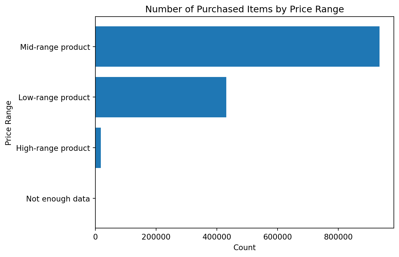

This chart is much easier to interpret than a raw histogram when the business question is about product segments rather than exact price values.

Example 2: Reorder Rate by price_range

reorder_by_price_range = (
    df_instacart
    .groupby("price_range")["reordered"]
    .mean()
    .sort_values()
)

reorder_by_price_range

price_range
High-range product    0.579092
Low-range product     0.590833
Mid-range product     0.602527
Not enough data       0.670455
Name: reordered, dtype: float64

reorder_by_price_range = (
    df_instacart
    .groupby("price_range")["reordered"]
    .mean()
    .sort_values()
)

plt.figure()
plt.barh(reorder_by_price_range.index, reorder_by_price_range.values)
plt.title("Reorder Rate by Price Range")
plt.xlabel("Reorder Rate")
plt.ylabel("Price Range")
plt.show()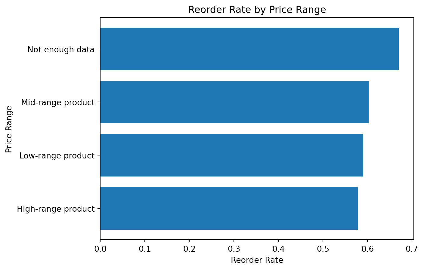

This is a good example of how a derived column can create a more business-oriented analytical story.

Example 3: Customer Counts by age_group

Because customer variables repeat at the product level, we first create a customer-level view.

df_customers_unique = df_instacart[
    ["First Name", "Surname", "Age", "income", "age_group", "income_group", "region"]
].drop_duplicates()

df_customers_unique.head()

	First Name	Surname	Age	income	age_group	income_group	region
0	Linda	Nguyen	31	40423	Middle	Middle income	South
11	Norma	Chapman	68	64940	Senior	Middle income	West
42	Janet	Lester	75	115242	Senior	High income	West
51	Peter	Villegas	39	89095	Middle	High income	Northeast
60	Anna	Allison	32	88603	Middle	High income	South

Now we can visualize the age groups.

age_group_counts = df_customers_unique["age_group"].value_counts().sort_values()
age_group_counts

age_group
Young     24682
Senior    44829
Middle    61698
Name: count, dtype: int64

age_group_counts = df_customers_unique["age_group"].value_counts().sort_values()

plt.figure()
plt.barh(age_group_counts.index, age_group_counts.values)
plt.title("Number of Customers by Age Group")
plt.xlabel("Count")
plt.ylabel("Age Group")
plt.show()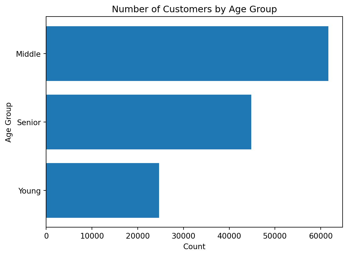

Example 4: Average Income by age_group

avg_income_by_age_group = (
    df_customers_unique
    .groupby("age_group")["income"]
    .mean()
    .sort_values()
)

avg_income_by_age_group

age_group
Young      67597.200065
Middle     94492.928247
Senior    109688.877356
Name: income, dtype: float64

avg_income_by_age_group = (
    df_customers_unique
    .groupby("age_group")["income"]
    .mean()
    .sort_values()
)

plt.figure()
plt.barh(avg_income_by_age_group.index, avg_income_by_age_group.values)
plt.title("Average Income by Age Group")
plt.xlabel("Average Income")
plt.ylabel("Age Group")
plt.show()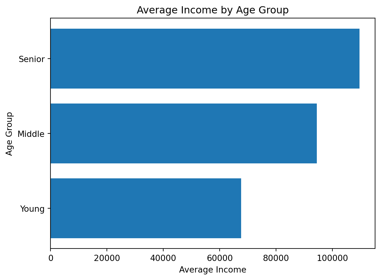

Example 5: Orders by order_time_band

Here we return to order-level analysis.

orders_time_band = (
    df_instacart[["order_id", "order_time_band"]]
    .drop_duplicates()
    .groupby("order_time_band")
    .size()
    .sort_values()
)

orders_time_band

order_time_band
Night         2507
Evening      24275
Morning      41068
Afternoon    63359
dtype: int64

orders_time_band = (
    df_instacart[["order_id", "order_time_band"]]
    .drop_duplicates()
    .groupby("order_time_band")
    .size()
    .sort_values()
)

plt.figure()
plt.barh(orders_time_band.index, orders_time_band.values)
plt.title("Number of Orders by Time Band")
plt.xlabel("Count")
plt.ylabel("Order Time Band")
plt.show()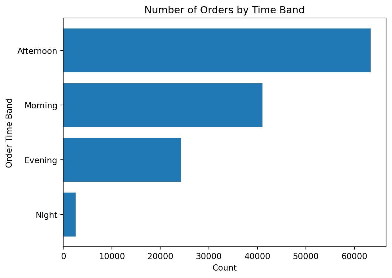

Practice Tasks

Task 1

Create a derived column called family_size_group based on n_dependants.

Suggested grouping:

• No dependants
• Small family
• Large family

Task 2

Create a derived column called senior_flag based on Age.

Suggested logic:

• Senior if age is 60 or more
• Not senior otherwise

Task 3

Visualize the number of customers by income_group.

Task 4

Visualize the reorder rate by order_time_band.

Task 5

Create a flag variable on dow using both lambda and isin() methods:

• weekend: True/1
• weekday: False/1