Session 13: Logistic Regression

Classification

Logistic Regression

Session Goal

In this session, we develop a complete understanding of logistic regression, starting from intuition and building up to implementation.

The focus is not only on the model itself, but on how it is used in real-world decision-making.

The key idea is:

Logistic regression connects data → probability → decision

Think of it as a pipeline:

We start with data about customers, users, or transactions
The model converts that data into a probability
That probability is then used to make a decision

For example:

A customer has a 0.82 probability of purchasing
Do we contact them or not?

This is where analytics meets business.

Introduction

Regression vs Classification

Before introducing logistic regression, we must clearly distinguish between two types of problems.

As we already know the Regression is used when the output is a continuous number:

predicting revenue
estimating house prices
forecasting demand

Example:

A customer is expected to spend $120 next month

Classification is used when the output is a category:

purchase vs not purchase
churn vs not churn
approve vs reject

Example:

Will the customer purchase? → Yes or No

This distinction is critical.

Why Regression is Misleading

Logistic regression is called “regression”, but it is actually used for classification problems.

\[\downarrow\]

Because it predicts probabilities, not categories directly.

Real Business Problems

Marketing Campaign

You have 1,000 customers $\rightarrow$ You want to send an offer $\rightarrow$ Each contact costs money

Question/Problem:

Who should we contact?

Telecom Churn

Customers may leave the service
Retention campaigns are expensive

Question/Problem:

Which customers are at risk of churning?

Loan Approval

Bank gives loans to customers
Some customers default

Question/Problem:

Should we approve this loan?

Important

All these problems are not just predictions, as they are decisions with consequences.

Binary Target Variable

In all these examples, the outcome has only two possible values.

\[ y \in \{0, 1\} \]

We encode outcomes as:

$1$ → event happens (purchase, churn, default)
$0$ → event does not happen

Example dataset:

Customer	Purchase
A	1
B	0
C	1

This encoding is essential because it allows us to work mathematically with classification.

Why Not Linear Regression?

The Problem

At first glance, you might think:

Why not just use linear regression?

We can try:

\[ \hat{y} = \beta_0 + \beta_1x \]

But here is the issue:

Linear regression can produce any value:

\[ -\infty < \hat{y} < +\infty \]

Why This Breaks for Classification

Suppose we predict:

$-0.3$ → does this make sense as probability?
$1.4$ → can probability be greater than 1?

$\downarrow$

No!

Probabilities must always satisfy:

\[ 0 \leq p \leq 1 \]

Imagine a marketing model predicts:

Customer A → 1.25 probability
Customer B → -0.15 probability

\[\downarrow\]

These outputs are meaningless.

This is why linear regression is not suitable for classification.

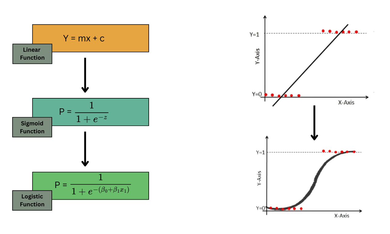
The Need for Transformation

Thus, we need a function that:

accepts any number from $-\infty$ to $+\infty$
always outputs a value between 0 and 1

This is exactly what the sigmoid function does.

From Probability to Decision

Predicting Probability

Logistic regression does not directly say:

“This customer will purchase”

Instead, it says:

\[ P(y = 1 \mid X) \]

Customer A → 0.82 probability of purchase

The probability gives us flexibility.

We can:

rank customers
prioritize actions
control risk

Threshold-Based Decision

To make a final decision, we use a threshold.

\[ \hat{y} = \begin{cases} 1, & p \geq 0.5 \\ 0, & p < 0.5 \end{cases} \]

Example table

Customer	Probability	Decision
A	0.82	1
B	0.63	1
C	0.47	0
D	0.12	0

Important to know

The threshold does not have to be 0.5.

In marketing → lower threshold (more aggressive)
In banking → higher threshold (more conservative)

Business translation:

Probability → level of confidence
Threshold → business strategy

This is where the model becomes actionable.

Logistic Regression Core Idea

Linear Score

Logistic regression starts similarly to linear regression.

We compute a score:

\[ z = \beta_0 + \beta_1x_1 + \cdots + \beta_kx_k \]

This is a weighted combination of features.

Example

Suppose:

\[ z = -2 + 0.6 \cdot \text{support calls} - 0.05 \cdot \text{tenure} \]

Interpretation (pay attention to signs):

more support calls → increases score
longer tenure → decreases score

Important

This score $z$ is not yet a probability.

It is just a position on a scale:

very negative → unlikely
around zero → uncertain
very positive → likely

Transition to Probability

To convert this score into a probability, we apply the sigmoid function:

\[ p = \frac{1}{1 + e^{-z}} \]

Intuition

Think of it like a decision system:

raw score → internal evaluation
sigmoid → converts into probability
threshold → converts into decision

	customer	raw_score	probability	decision
0	Customer A	-4.0	0.017986	No Churn
1	Customer B	-1.5	0.182426	No Churn
2	Customer C	0.0	0.500000	Churn
3	Customer D	1.5	0.817574	Churn
4	Customer E	4.0	0.982014	Churn

Mini Example

If:

\[ z = 0 \]

then:

\[ p = 0.5 \]

If:

\[ z = 2 \]

then:

\[ p \approx 0.88 \]

If:

\[ z = -2 \]

then:

\[ p \approx 0.12 \]

Important

Logistic regression works in three steps:

Compute a score $z$
Convert score into probability $p$
Apply threshold to make decision

This completes the conceptual foundation before moving into implementation.

Storytelling Perspective

Imagine a telecom company evaluating customers for churn.

Each customer gets a score:

many complaints → increases score
long tenure → decreases score
high monthly charges → increases score

So:

Customer A → $z = -3.2$ → very unlikely to churn
Customer B → $z = 0.4$ → uncertain
Customer C → $z = 2.1$ → very likely to churn

But these are just scores, not probabilities.

Intuition Through Examples

Let’s examine how different values of $z$ behave.

import numpy as np
import pandas as pd

z_values = [-5, -2, -1, 0, 1, 2, 5]
p_values = 1 / (1 + np.exp(-np.array(z_values)))

df_sigmoid = pd.DataFrame({
    "score_z": z_values,
    "probability": p_values
})

df_sigmoid

	score_z	probability
0	-5	0.006693
1	-2	0.119203
2	-1	0.268941
3	0	0.500000
4	1	0.731059
5	2	0.880797
6	5	0.993307

Interpretation

Score ($z$)	Probability
very negative	close to 0
0	0.5
very positive	close to 1

Logistic regression is not linear in probability — it is linear in log-odds

Understanding Odds

From Probability to Odds

Instead of working directly with probability, logistic regression uses odds:

\[ \text{odds} = \frac{p}{1-p} \]

Example 1:

If:

\[ p = 0.75 \]

then:

\[ \text{odds} = \frac{0.75}{0.25} = 3 \]

Interpretation:

The event is 3 times more likely to happen than not happen

Example 2: Winning Game

Sayin that the odds in favor of my team (FC Barcelona) winning a game are 4 to 1 means:

4 of 5 times they win
1 of 5 times they lose.

Example 3: Lossing Game

Sayin that the odds in favor of my team (Real Madrid) winning a game are 1 to 4 means:

1 of 5 times they win
4 of 5 times they lose.

Odds Table

probabilities = [0.1, 0.3, 0.5, 0.7, 0.9]

odds_table = pd.DataFrame({
    "probability": probabilities
})

odds_table["odds"] = odds_table["probability"] / (1 - odds_table["probability"])

odds_table

	probability	odds
0	0.1	0.111111
1	0.3	0.428571
2	0.5	1.000000
3	0.7	2.333333
4	0.9	9.000000

Important

probability increases linearly
odds increase non-linearly

This makes odds more suitable for modeling.

From Odds to Log-Odds

Why Take the Log?

Odds are always positive:

\[ 0 < \text{odds} < \infty \]

But we want a model that can handle:

\[ -\infty < \text{value} < +\infty \]

So we take the logarithm:

\[ \log\left(\frac{p}{1-p}\right) \]

This is called the log-odds or logit.

Logistic Regression Equation

Now we connect everything: Logistic regression models the log-odds as a linear function of features:

\[ \log\left(\frac{p}{1-p}\right) = \beta_0 + \beta_1x_1 + \cdots + \beta_kx_k \]

This equation tells us:

Each feature changes the log-odds, not the probability directly

Interpreting Coefficients Properly

Direction of Effect

$\beta > 0$ → increases probability
$\beta < 0$ → decreases probability

Magnitude via Odds Ratio

To interpret magnitude, we use:

\[ e^{\beta} \]

sometimes called the odds ratio or exp($\beta$).

Example

If:

\[ \beta = 0.7 \]

then:

\[ e^{0.7} \approx 2.01 \]

\[\downarrow\]

A one-unit increase in this feature doubles the odds of the event

Business Translation

Suppose:

feature = number of support calls
coefficient = 0.7
$e^{0.7} \approx 2$

Then:

Each additional support call doubles the odds of churn

Bringing Everything Together

Logistic regression works as a pipeline:

Step 1 | Linear Score

\[ z = \beta_0 + \beta_1x_1 + \cdots \]

Step 2 | Convert to Probability

\[ p = \frac{1}{1 + e^{-z}} \]

Step 3 | Make Decision

\[ \hat{y} = \begin{cases} 1, & p \geq \text{threshold} \\ 0, & p < \text{threshold} \end{cases} \]

Test your understanding | Odds

Question 1 | Probability to Odds

A customer has a 60% probability of churn.

What are the odds of churn?
Interpret the result

Question 2 | Log-Odds to Probability

A model gives:

\[ \log(\text{odds}) = 2 \]

Convert to odds
Convert to probability
Interpret the result

Question 1 | Solution

Recall:

\[ \text{odds} = \frac{p}{1-p} \]

\[ p = 0.6 \]

\[ \text{odds} = \frac{0.6}{0.4} = 1.5 \]

Interpretation:

The event is 1.5 times more likely to happen than not happen
Churn is more likely than staying, but not extremely strong

Question 2 | Solution

Recall:

\[ \text{odds} = e^{\text{log-odds}} \]

\[ \text{odds} = e^2 \approx 7.39 \]

Now convert to probability:

\[ p = \frac{7.39}{1 + 7.39} \approx 0.88 \]

Interpretation:

The probability is approximately 88%
This represents a very high likelihood of the event

Final Intuition

The model builds a score
The sigmoid converts it into probability
The threshold converts it into action

Logistic regression is not about predicting 0 or 1
It is about estimating how likely something is to happen

This is what makes it powerful for real-world decision systems.

Video Explanation

Check out this video for a visual explanation of logistic regression:

Odd Ratios and Log-Odds Explained | Logistic Regression Intuition

Case Study 1: Customer Churn Prediction

In this section, we will use sythetic data to illustrate the entire logistic regression pipeline.

train a logistic regression model
interpret results using:
- coefficients and $e^{\beta}$
- confusion matrix
- revenue matrix

Download the Dataset

import pandas as pd

import numpy as np
import pandas as pd

from sklearn.model_selection import train_test_split
from sklearn.linear_model import LogisticRegression
from sklearn.metrics import confusion_matrix, accuracy_score, precision_score, recall_score, f1_score

df = pd.read_csv("https://raw.githubusercontent.com/hovhannisyan91/data_analytics_with_python/refs/heads/main/data/regression/logistic_regression/synthetic_churn_data.csv")
print(f"Dataset shape: {df.shape}")
df.head()


df.to_csv("../../lab/python/data/regression/logistic_regression/synthetic_churn_data.csv", index=False)

Dataset shape: (1000, 6)

Observing the Dataframe

Before modeling, we should always inspect the dataset.

df.info()

<class 'pandas.DataFrame'>
RangeIndex: 1000 entries, 0 to 999
Data columns (total 6 columns):
 #   Column           Non-Null Count  Dtype  
---  ------           --------------  -----  
 0   tenure           1000 non-null   int64  
 1   monthly_charges  1000 non-null   float64
 2   support_calls    1000 non-null   int64  
 3   contract_type    1000 non-null   int64  
 4   churn            1000 non-null   int64  
 5   education_level  1000 non-null   str    
dtypes: float64(1), int64(4), str(1)
memory usage: 53.8 KB

The dataset now contains both numeric and categorical variables.

Column	Meaning
`tenure`	Number of months the customer has stayed with the company
`monthly_charges`	Monthly amount paid by the customer
`support_calls`	Number of support calls made by the customer
`contract_type`	Contract type, where 0 = prepaid and 1 = postpaid
`education_level`	Customer education category
`churn`	Target variable, where 1 = churn and 0 = no churn

The target variable is:

\[ y = \text{churn} \]

where:

1: customer churned (left the service)
0: customer did not churn (stayed with the service)

Exploratory Data Analysis

Target Variable Distribution

df['churn'].value_counts(normalize=True)

churn
0    0.633
1    0.367
Name: proportion, dtype: float64

Churn Rate by Contract Type

churn_rate_by_contract = df.groupby('contract_type')['churn'].mean().reset_index()
import plotly.express as px
fig = px.bar(churn_rate_by_contract, x='contract_type', y='churn', title='Churn Rate by Contract Type')
fig.update_layout(
    xaxis_title='Contract Type (0 = Prepaid, 1 = Postpaid',
    yaxis_title='Churn Rate',
    template='plotly_white'
)   
fig.show()

As it was expected, the churn rate is lower for postpaid customers (contract_type = 1) compared to prepaid customers (contract_type = 0).

Tip

Think about why this might be the case. What are the possible reasons for this difference in churn rates between prepaid and postpaid customers?

Churn Rate by Education Level

churn_rate_by_education = df.groupby('education_level')['churn'].mean().reset_index()
import plotly.express as px
fig = px.bar(churn_rate_by_education, x='education_level', y='churn', title='Churn Rate by Education Level')
fig.update_layout(
    xaxis_title='Education Level',
    yaxis_title='Churn Rate',
    template='plotly_white'
)   
fig.show()

The lowest observed churn rate is 12.40%.
The highest observed churn rate is 63.60%.

Data Preprocessing

We now separate the dataset into input variables and the target variable.

X = df.drop(columns=["churn"])
y = df["churn"]

X: contains all the features that we will use to predict churn
y contains the target variable indicating whether a customer churned or not.

Encoding Categorical Variables

Logistic regression (basically all the ML models) requires numeric input.

The column education_level contains text categories, so we convert it into dummy variables.

Beofre encoding, the education_level column has 4 categories: and we will create 3 new binary columns to represent these categories (dropping one to avoid multicollinearity). As a base category, we will use education_level = "High School".

In ordert to make sure that the baseiline category is we will enforce the category using pd.Categorical before encoding.

education_order = ["High School", "Bachelor", "Master", "PhD"]

df["education_level"] = pd.Categorical(
    df["education_level"],
    categories=education_order,
    ordered=True
)

education_dummies = pd.get_dummies(
    df["education_level"],
    prefix="education",
    drop_first=True,
    dtype=int
)

education_dummies.head()

	education_Bachelor	education_Master
0	0	0
1	1	0
2	0	1
3	0	0
4	0	1

The remaining dummy variables compare each education level against that baseline.

For example, if the baseline is High School, then:

Dummy Variable	Interpretation
`education_level_Bachelor`	Bachelor compared with High School
`education_level_Master`	Master compared with High School
`education_level_PhD`	PhD compared with High School

Once we have the dummy variables, we can concatenate them back to the original dataframe and drop the original education_level column. Pay attention to the axis=1, which indicates that we are concatenating columns (not rows).

X_encoded = pd.concat([X.drop(columns=["education_level"]), education_dummies], axis=1)

X_encoded.head()

	tenure	monthly_charges	support_calls	contract_type	education_Bachelor	education_Master
0	29	46.867736	6	0	0	0
1	15	74.163421	6	0	1	0
2	8	83.347822	3	1	0	1
3	21	45.788769	2	0	0	0
4	19	33.935607	7	0	0	1

Checking the final set of features

print("Final set of features:")
print(X_encoded.dtypes)

Final set of features:
tenure                  int64
monthly_charges       float64
support_calls           int64
contract_type           int64
education_Bachelor      int64
education_Master        int64
education_PhD           int64
dtype: object

Making sure that all the features are numeric is crucial for the logistic regression model to work properly. If there were any remaining categorical variables, we would need to encode them as well before proceeding with modeling.

Train-Test Split

Before training the model, we divide the data into two parts:

Training set
Test set

The training set is used to teach the model.
The test set is used to evaluate whether the model can make good predictions on new, unseen data

X_train, X_test, y_train, y_test = train_test_split(
    X_encoded,
    y,
    test_size=0.2,
    random_state=42,
    stratify=y
)

In machine learning, we should not evaluate the model on the same data that was used for training.

If we train and test the model on the same dataset, the model may appear to perform very well simply because it has already seen those examples. This does not tell us whether the model can generalize to new customers.

The train-test split helps us answer the following question:

Can the model make accurate predictions for customers it has not seen before?

For example, if we have 1,000 customers, using test_size=0.2 means:

Dataset Part	Percentage	Number of Customers
Training set	80%	800
Test set	20%	200

The model learns from the training set and is evaluated on the test set.

`random_state=42`

The train-test split is random by default.

This means that every time we run the code, Python may select different rows for the training and test sets.

As a result, the model results may slightly change every time we run the notebook.

By setting:

random_state=42

we make the split reproducible.

This means that every time we run the code, we get the same training and testing sets.

The number 42 is not mathematically special. It is simply a commonly used fixed number.

`stratify=y`

The argument stratify=y is very important for classification problems.

It tells Python to preserve the same class distribution in both the training set and the test set.

For example, suppose the full dataset has the following churn distribution:

Class	Meaning	Percentage
0	Did not churn	80%
1	Churned	20%

With stratify=y, the training and test sets will keep approximately the same balance:

Dataset Part	Did Not Churn	Churned
Training set	80%	20%
Test set	80%	20%

This is especially important when the target variable is imbalanced.

In churn prediction, the number of customers who churn is usually much smaller than the number of customers who do not churn.

Without stratification, the test set may accidentally contain too few churned customers or too many churned customers.

That would make the model evaluation unreliable.

For example, if the test set contains very few churned customers, the model may look better than it really is.

Output of `train_test_split()`

The function returns four objects:

X_train, X_test, y_train, y_test

Each one has a specific purpose.

X_train: contains the input features for the training data. This is the data the model uses to learn patterns.
X_test: contains the input features for the test data. This allows us to test how well the model performs on unseen customers.
y_train: contains the true target values for the training data. This is what the model tries to predict during training.
y_test: contains the true target values for the test data. This is what we use to evaluate the model’s predictions on the test set.

Let’s check the shapes of these objects to confirm that the split was done correctly.

train_size = len(X_train)
test_size = len(X_test)

train_churn_rate = y_train.mean()
test_churn_rate = y_test.mean()

print("Training rows:", train_size)
print("Test rows:", test_size)
print("Training churn rate:", round(train_churn_rate, 3))
print("Test churn rate:", round(test_churn_rate, 3))

Training rows: 800
Test rows: 200
Training churn rate: 0.368
Test churn rate: 0.365

Thus , the train-test split is used to check whether the model can generalize.

The training set contains 800 customers.

The test set contains 200 customers.

The churn rate in the training set is np.float64(36.75)%, while the churn rate in the test set is np.float64(36.5)%.

Because we used stratification, these two percentages should be close.

Training the Logistic Regression Model

model = LogisticRegression(max_iter=1000)

model.fit(X_train, y_train)

LogisticRegression(max_iter=1000)

In a Jupyter environment, please rerun this cell to show the HTML representation or trust the notebook.
On GitHub, the HTML representation is unable to render, please try loading this page with nbviewer.org.

max_iter=1000 is used to ensure that the optimization algorithm has enough iterations to converge to a solution. Logistic regression uses an iterative process to find the best coefficients, and sometimes it may require more iterations than the default (which is usually 100) to find the optimal solution, especially if the dataset is complex or has many features.

The model estimates coefficients for each feature.

Internally, logistic regression models the log-odds of churn:

\[ \log\left(\frac{p}{1-p}\right) = \beta_0 + \beta_1x_1 + \cdots + \beta_kx_k \]

where $p$ is the probability of churn.

Predicting Probabilities on the Test Set

probs = model.predict_proba(X_test)
probs[:5]

array([[0.98318855, 0.01681145],
       [0.58272749, 0.41727251],
       [0.52510491, 0.47489509],
       [0.3840094 , 0.6159906 ],
       [0.67936502, 0.32063498]])

The output probs contains the predicted probability of churn for each customer in the test set.

We use [:, 1] because class 1 represents churn.

probs = probs[:, 1]
probs[:5]

array([0.01681145, 0.41727251, 0.47489509, 0.6159906 , 0.32063498])

Converting the Probabilities into Binary Predictions

threshold = 0.5
preds = (probs >= threshold).astype(int)
preds[:5]

array([0, 0, 0, 1, 0])

The threshold converts probabilities into class predictions.

\[ \hat{y} = \begin{cases} 1, & p \geq 0.5 \\ 0, & p < 0.5 \end{cases} \]

Previewing the Predictions

prediction_results = X_test.copy()

prediction_results["actual_churn"] = y_test.values
prediction_results["predicted_probability"] = probs
prediction_results["predicted_churn"] = preds

prediction_results.head()

	tenure	monthly_charges	support_calls	contract_type	education_Master	education_PhD	actual_churn	predicted_probability	predicted_churn
361	34	55.062693	2	1	0	0	0	0.016811	0
5	23	103.493024	4	0	0	1	0	0.417273	0
692	25	75.778342	5	0	1	0	1	0.474895	0
708	6	112.717782	5	1	1	0	0	0.615991	1
841	26	67.601813	7	1	0	1	0	0.320635	0

Coefficient Interpretation with Exponentiated Betas

The raw coefficients are log-odds coefficients.

To make them easier to interpret, we exponentiate them.

coef_df = pd.DataFrame({
    "feature": X_encoded.columns,
    "beta": model.coef_[0],
    "exp_beta": np.exp(model.coef_[0])
})

coef_df = coef_df.sort_values("exp_beta", ascending=False)

coef_df

	feature	beta	exp_beta
2	support_calls	0.569350	1.767118
4	education_Bachelor	0.122790	1.130646
5	education_Master	0.112264	1.118808
1	monthly_charges	0.020344	1.020552
0	tenure	-0.055288	0.946213
6	education_PhD	-0.226263	0.797508
3	contract_type	-1.228894	0.292616

Interpretation

The table contains two important values:

Column	Meaning
`beta`	Effect on log-odds
`exp_beta`	Odds multiplier, calculated as $e^{\beta}$

Rules for interpretation:

If exp_beta > 1, the feature increases the odds of churn
If exp_beta < 1, the feature decreases the odds of churn
If exp_beta = 1, the feature has almost no effect on churn odds

Support Calls

exp_beta = 1.77
Each additional support call multiplies churn odds by 1.77
This means churn odds increase by approximately 77%
This is the strongest churn-increasing factor

Business meaning: frequent support calls are an early warning signal

Education: Bachelor

exp_beta = 1.13
Bachelor customers have 1.13 times the odds of churn compared with the baseline education group
This means approximately 13% higher odds of churn

The effect is positive but relatively small

Education: Master

exp_beta = 1.12
Master customers have 1.12 times the odds of churn compared with the baseline education group
This means approximately 12% higher odds of churn

The effect is also positive but relatively small

Education: PhD

exp_beta = 0.80
PhD customers have 0.80 times the odds of churn compared with the baseline education group
This means approximately 20% lower odds of churn
This result goes against the original assumption that higher education should always increase churn risk

Possible reason: other variables may explain churn better, or the synthetic relationship may not be strong enough

Monthly Charges

exp_beta = 1.02
Each one-unit increase in monthly charges multiplies churn odds by 1.02
This means approximately 2% higher odds of churn per unit
The single-unit effect is small, but larger price differences can matter

Example:

\[ 1.02^{10} \approx 1.22 \]

A 10-unit increase in monthly charges is associated with roughly 22% higher odds of churn.

Tenure

exp_beta = 0.95
Each additional month of tenure multiplies churn odds by 0.95
This means churn odds decrease by approximately 5% per month

Business meaning: longer-tenure customers are more stable

Contract Type

exp_beta = 0.29
Postpaid contract customers have 0.29 times the odds of churn compared with prepaid customers
This means approximately 71% lower odds of churn
This is the strongest churn-reducing factor

Business meaning: long-term contracts strongly reduce churn risk

Retention Strategy

The company should prioritize customers who:

have many support calls
pay higher monthly charges
have short tenure
are on postpaid contracts

These customers are more likely to churn and are good candidates for retention campaigns.

Confusion Matrix

One of the most common ways to evaluate classification models is through the confusion matrix.

The confusion matrix compares actual churn outcomes with predicted churn outcomes.

Outcome	Meaning
True Positive	Customer churned and model predicted churn
False Positive	Customer did not churn but model predicted churn
False Negative	Customer churned but model missed it
True Negative	Customer did not churn and model predicted no churn

cm = confusion_matrix(y_test, preds)

tn, fp, fn, tp = cm.ravel()

cm

array([[103,  24],
       [ 23,  50]])

Classification Metrics

accuracy = accuracy_score(y_test, preds)
precision = precision_score(y_test, preds)
recall = recall_score(y_test, preds)

print("Accuracy:", round(accuracy, 3))
print("Precision:", round(precision, 3))
print("Recall:", round(recall, 3))

Accuracy: 0.765
Precision: 0.676
Recall: 0.685

Accuracy

The model accuracy is 76.5%.

Precision

The precision is 67.57%.

This means that among customers predicted as churners, 67.57% actually churned.

Recall

The recall is 68.49%.

This means that among all actual churners, the model identified 68.49%.

ROC Curve and AUC

After using the confusion matrix, we can also evaluate the logistic regression (all the available classification models) model using the ROC curve (Receiver Operating Characteristic) and the AUC (Area Under the Curve).

ROC Intuition

The confusion matrix depends on one selected threshold.

For example:

threshold = 0.5

But in business problems, the threshold may change depending on the strategy.

For churn prediction:

lower threshold → contact more customers
higher threshold → contact fewer customers
lower threshold may increase recall
higher threshold may increase precision

The ROC curve helps us understand how the model behaves across different threshold values.

ROC Curve

The ROC curve compares two quantities:

Metric	Meaning
True Positive Rate	How many actual churners we correctly identify
False Positive Rate	How many non-churners we incorrectly classify as churners

The formulas are:

\[ TPR = \frac{TP}{TP + FN} \]

\[ FPR = \frac{FP}{FP + TN} \]

In churn language:

TPR answers: among customers who actually churned, how many did we detect?
FPR answers: among customers who did not churn, how many did we incorrectly target?

ROC Curve Code

from sklearn.metrics import roc_curve, roc_auc_score
import matplotlib.pyplot as plt

fpr, tpr, thresholds = roc_curve(y_test, probs)

auc_score = roc_auc_score(y_test, probs)

plt.figure(figsize=(8, 6))
plt.plot(fpr, tpr, label=f"ROC Curve (AUC = {auc_score:.3f})")
plt.plot([0, 1], [0, 1], linestyle="--", label="Random Model")

plt.xlabel("False Positive Rate")
plt.ylabel("True Positive Rate")
plt.title("ROC Curve for Logistic Regression Model")
plt.legend()
plt.grid(True)
plt.show()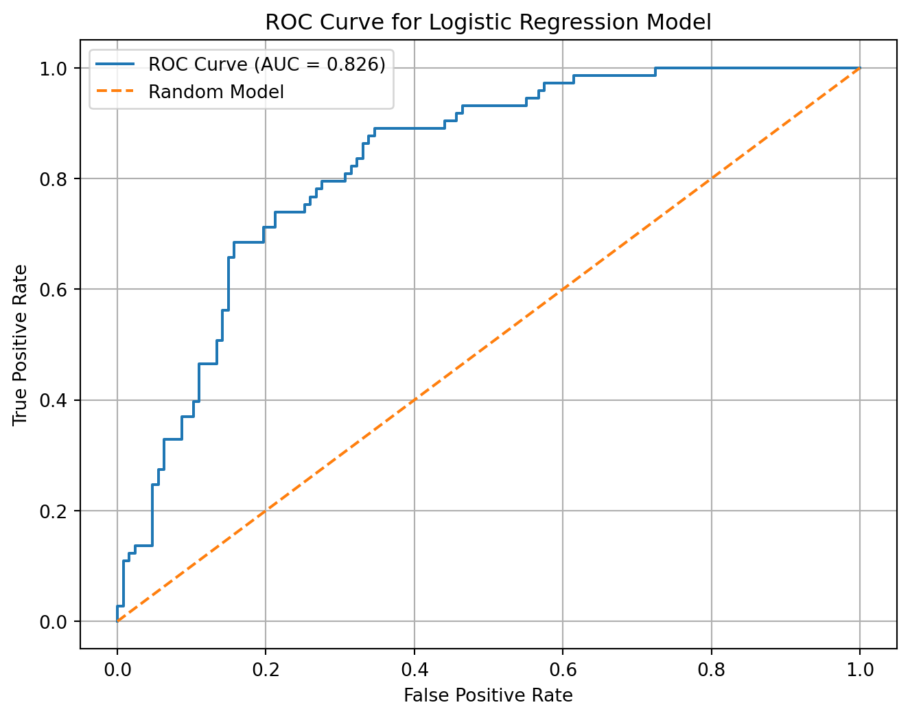

The model AUC is 0.826.

This means that the model has a 82.56% ability to rank a randomly selected churner higher than a randomly selected non-churner.

How to Interpret AUC

AUC Value	Interpretation
0.50	No better than random guessing
0.60–0.70	Weak model
0.70–0.80	Acceptable model
0.80–0.90	Strong model
0.90+	Very strong model

Business Interpretation

If AUC is close to 0.5, the model cannot separate churners from non-churners well
If AUC is high, the model is good at ranking customers by churn risk
A high AUC does not automatically mean the campaign is profitable

We still need the confusion matrix and revenue matrix to choose the best threshold

Threshold Table from ROC Curve

The ROC curve gives many possible thresholds.

We can inspect some of them:

roc_threshold_table = pd.DataFrame({
    "threshold": thresholds,
    "false_positive_rate": fpr,
    "true_positive_rate": tpr
})

roc_threshold_table.head(10)

	threshold	false_positive_rate	true_positive_rate
0	inf	0.000000	0.000000
1	0.942007	0.000000	0.013699
2	0.918466	0.000000	0.027397
3	0.914077	0.007874	0.027397
4	0.872713	0.007874	0.109589
5	0.865498	0.015748	0.109589
6	0.864796	0.015748	0.123288
7	0.863052	0.023622	0.123288
8	0.856353	0.023622	0.136986
9	0.836171	0.047244	0.136986

Summary

The ROC curve evaluates model ranking ability.
The revenue matrix evaluates business value.

\[\downarrow\]

ROC/AUC tells us whether the model separates churners from non-churners
Confusion matrix tells us the classification results at one threshold
Revenue matrix tells us whether the classification strategy creates profit

Revenue Matrix

There is a cost associated with contacting customers and a cost associated with losing customers. Usally from Data Analytics perspective, we want to maximize revenue, not just accuracy. Revenue matrix allows us to evaluate the model based on the financial impact of its predictions.

Assume the company contacts customers predicted as likely to churn.

retention_cost = 10
retention_benefit = 50

revenue_from_saved_customers = tp * (retention_benefit - retention_cost)
cost_from_unnecessary_contacts = fp * retention_cost

net_profit = revenue_from_saved_customers - cost_from_unnecessary_contacts

print("Revenue from saved customers:", revenue_from_saved_customers)
print("Cost from unnecessary contacts:", cost_from_unnecessary_contacts)
print("Net profit:", net_profit)

Revenue from saved customers: 2000
Cost from unnecessary contacts: 240
Net profit: 1760

Prediction Outcome	Business Meaning	Financial Effect
True Positive	Correctly targeted churner	`retention_benefit - retention_cost`
False Positive	Contacted non-churner unnecessarily	`-retention_cost`
False Negative	Missed churner	`0`
True Negative	Correctly ignored non-churner	`0`

The model correctly targeted np.int64(50) churners.

These customers generated np.int64(2000) units of value after subtracting campaign cost.

The model also contacted np.int64(24) customers unnecessarily, creating a cost of np.int64(240).

The final estimated campaign profit is np.int64(1760).

Homework: Customer Churn Prediction

Use the same steps to build a logistic regression model on the customer_churn_data.csv dataset.

df = pd.read_csv("https://raw.githubusercontent.com/hovhannisyan91/data_analytics_with_python/refs/heads/main/data/regression/logistic_regression/Telco_Customer_Churn.csv")
df.head()

	customerID	gender	Partner	Dependents	tenure	PhoneService	MultipleLines	InternetService	OnlineSecurity	...	DeviceProtection	TechSupport	StreamingTV	StreamingMovies	Contract	PaperlessBilling	PaymentMethod	MonthlyCharges	TotalCharges	Churn
0	7590-VHVEG	Female	Yes	No	1	No	No phone service	DSL	No	...	No	No	No	No	Month-to-month	Yes	Electronic check	29.85	29.85	No
1	5575-GNVDE	Male	No	No	34	Yes	No	DSL	Yes	...	Yes	No	No	No	One year	No	Mailed check	56.95	1889.5	No
2	3668-QPYBK	Male	No	No	2	Yes	No	DSL	Yes	...	No	No	No	No	Month-to-month	Yes	Mailed check	53.85	108.15	Yes
3	7795-CFOCW	Male	No	No	45	No	No phone service	DSL	Yes	...	Yes	Yes	No	No	One year	No	Bank transfer (automatic)	42.30	1840.75	No
4	9237-HQITU	Female	No	No	2	Yes	No	Fiber optic	No	...	No	No	No	No	Month-to-month	Yes	Electronic check	70.70	151.65	Yes

5 rows × 21 columns

We have customer information for a Telecommunications company:

We’ve got customer IDs, general customer info, the servies they’ve subscribed too, type of contract and monthly charges. This is a historic customer information so we have a field stating whether that customer has churned

Field Descriptions:

customerID - Customer ID
gender - Whether the customer is a male or a female
SeniorCitizen - Whether the customer is a senior citizen or not (1, 0)
Partner - Whether the customer has a partner or not (Yes, No)
Dependents - Whether the customer has dependents or not (Yes, No)
tenure - Number of months the customer has stayed with the company
PhoneService - Whether the customer has a phone service or not (Yes, No)
MultipleLines - Whether the customer has multiple lines or not (Yes, No, No phone service)
InternetService - Customer’s internet service provider (DSL, Fiber optic, No)
OnlineSecurity - Whether the customer has online security or not (Yes, No, No internet service)
OnlineBackup - Whether the customer has online backup or not (Yes, No, No internet service)
DeviceProtection - Whether the customer has device protection or not (Yes, No, No internet service)
TechSupport - Whether the customer has tech support or not (Yes, No, No internet service)
StreamingTV - Whether the customer has streaming TV or not (Yes, No, No internet service)
StreamingMovies - Whether the customer has streaming movies or not (Yes, No, No internet service)
Contract - The contract term of the customer (Month-to-month, One year, Two year)
PaperlessBilling - Whether the customer has paperless billing or not (Yes, No)
PaymentMethod - The customer’s payment method (Electronic check, Mailed check Bank transfer (automatic), Credit card (automatic))
MonthlyCharges - The amount charged to the customer monthly
TotalCharges - The total amount charged to the customer
Churn - Whether the customer churned or not (Yes or No)

	penalty penalty: {'l1', 'l2', 'elasticnet', None}, default='l2' Specify the norm of the penalty: - `None`: no penalty is added; - `'l2'`: add a L2 penalty term and it is the default choice; - `'l1'`: add a L1 penalty term; - `'elasticnet'`: both L1 and L2 penalty terms are added. .. warning:: Some penalties may not work with some solvers. See the parameter `solver` below, to know the compatibility between the penalty and solver. .. versionadded:: 0.19 l1 penalty with SAGA solver (allowing 'multinomial' + L1) .. deprecated:: 1.8 `penalty` was deprecated in version 1.8 and will be removed in 1.10. Use `l1_ratio` instead. `l1_ratio=0` for `penalty='l2'`, `l1_ratio=1` for `penalty='l1'` and `l1_ratio` set to any float between 0 and 1 for `'penalty='elasticnet'`.	'deprecated'
	C C: float, default=1.0 Inverse of regularization strength; must be a positive float. Like in support vector machines, smaller values specify stronger regularization. `C=np.inf` results in unpenalized logistic regression. For a visual example on the effect of tuning the `C` parameter with an L1 penalty, see: :ref:`sphx_glr_auto_examples_linear_model_plot_logistic_path.py`.	1.0
	l1_ratio l1_ratio: float, default=0.0 The Elastic-Net mixing parameter, with `0 <= l1_ratio <= 1`. Setting `l1_ratio=1` gives a pure L1-penalty, setting `l1_ratio=0` a pure L2-penalty. Any value between 0 and 1 gives an Elastic-Net penalty of the form `l1_ratio * L1 + (1 - l1_ratio) * L2`. .. warning:: Certain values of `l1_ratio`, i.e. some penalties, may not work with some solvers. See the parameter `solver` below, to know the compatibility between the penalty and solver. .. versionchanged:: 1.8 Default value changed from None to 0.0. .. deprecated:: 1.8 `None` is deprecated and will be removed in version 1.10. Always use `l1_ratio` to specify the penalty type.	0.0
	dual dual: bool, default=False Dual (constrained) or primal (regularized, see also :ref:`this equation `) formulation. Dual formulation is only implemented for l2 penalty with liblinear solver. Prefer `dual=False` when n_samples > n_features.	False
	tol tol: float, default=1e-4 Tolerance for stopping criteria.	0.0001
	fit_intercept fit_intercept: bool, default=True Specifies if a constant (a.k.a. bias or intercept) should be added to the decision function.	True
	intercept_scaling intercept_scaling: float, default=1 Useful only when the solver `liblinear` is used and `self.fit_intercept` is set to `True`. In this case, `x` becomes `[x, self.intercept_scaling]`, i.e. a "synthetic" feature with constant value equal to `intercept_scaling` is appended to the instance vector. The intercept becomes ``intercept_scaling * synthetic_feature_weight``. .. note:: The synthetic feature weight is subject to L1 or L2 regularization as all other features. To lessen the effect of regularization on synthetic feature weight (and therefore on the intercept) `intercept_scaling` has to be increased.	1
	class_weight class_weight: dict or 'balanced', default=None Weights associated with classes in the form ``{class_label: weight}``. If not given, all classes are supposed to have weight one. The "balanced" mode uses the values of y to automatically adjust weights inversely proportional to class frequencies in the input data as ``n_samples / (n_classes * np.bincount(y))``. Note that these weights will be multiplied with sample_weight (passed through the fit method) if sample_weight is specified. .. versionadded:: 0.17 class_weight='balanced'	None
	random_state random_state: int, RandomState instance, default=None Used when ``solver`` == 'sag', 'saga' or 'liblinear' to shuffle the data. See :term:`Glossary ` for details.	None
	solver solver: {'lbfgs', 'liblinear', 'newton-cg', 'newton-cholesky', 'sag', 'saga'}, default='lbfgs' Algorithm to use in the optimization problem. Default is 'lbfgs'. To choose a solver, you might want to consider the following aspects: - 'lbfgs' is a good default solver because it works reasonably well for a wide class of problems. - For :term:`multiclass` problems (`n_classes >= 3`), all solvers except 'liblinear' minimize the full multinomial loss, 'liblinear' will raise an error. - 'newton-cholesky' is a good choice for `n_samples` >> `n_features * n_classes`, especially with one-hot encoded categorical features with rare categories. Be aware that the memory usage of this solver has a quadratic dependency on `n_features * n_classes` because it explicitly computes the full Hessian matrix. - For small datasets, 'liblinear' is a good choice, whereas 'sag' and 'saga' are faster for large ones; - 'liblinear' can only handle binary classification by default. To apply a one-versus-rest scheme for the multiclass setting one can wrap it with the :class:`~sklearn.multiclass.OneVsRestClassifier`. .. warning:: The choice of the algorithm depends on the penalty chosen (`l1_ratio=0` for L2-penalty, `l1_ratio=1` for L1-penalty and `0 < l1_ratio < 1` for Elastic-Net) and on (multinomial) multiclass support: ================= ======================== ====================== solver l1_ratio multinomial multiclass ================= ======================== ====================== 'lbfgs' l1_ratio=0 yes 'liblinear' l1_ratio=1 or l1_ratio=0 no 'newton-cg' l1_ratio=0 yes 'newton-cholesky' l1_ratio=0 yes 'sag' l1_ratio=0 yes 'saga' 0<=l1_ratio<=1 yes ================= ======================== ====================== .. note:: 'sag' and 'saga' fast convergence is only guaranteed on features with approximately the same scale. You can preprocess the data with a scaler from :mod:`sklearn.preprocessing`. .. seealso:: Refer to the :ref:`User Guide ` for more information regarding :class:`LogisticRegression` and more specifically the :ref:`Table ` summarizing solver/penalty supports. .. versionadded:: 0.17 Stochastic Average Gradient (SAG) descent solver. Multinomial support in version 0.18. .. versionadded:: 0.19 SAGA solver. .. versionchanged:: 0.22 The default solver changed from 'liblinear' to 'lbfgs' in 0.22. .. versionadded:: 1.2 newton-cholesky solver. Multinomial support in version 1.6.	'lbfgs'
	max_iter max_iter: int, default=100 Maximum number of iterations taken for the solvers to converge.	1000
	verbose verbose: int, default=0 For the liblinear and lbfgs solvers set verbose to any positive number for verbosity.	0
	warm_start warm_start: bool, default=False When set to True, reuse the solution of the previous call to fit as initialization, otherwise, just erase the previous solution. Useless for liblinear solver. See :term:`the Glossary `. .. versionadded:: 0.17 warm_start to support lbfgs, newton-cg, sag, saga solvers.	False
	n_jobs n_jobs: int, default=None Does not have any effect. .. deprecated:: 1.8 `n_jobs` is deprecated in version 1.8 and will be removed in 1.10.	None

Session Goal

Introduction

Regression vs Classification

Real Business Problems

Binary Target Variable

Why Not Linear Regression?

The Problem

Why This Breaks for Classification

The Need for Transformation

From Probability to Decision

Predicting Probability

Threshold-Based Decision

Logistic Regression Core Idea

Linear Score

Example

Transition to Probability

Intuition

Mini Example

Storytelling Perspective

Intuition Through Examples

Interpretation

Understanding Odds

From Probability to Odds

Example 1:

Example 2: Winning Game

Example 3: Lossing Game

Odds Table

From Odds to Log-Odds

Logistic Regression Equation

Interpreting Coefficients Properly

Direction of Effect

Magnitude via Odds Ratio

Example

Business Translation

Bringing Everything Together

Step 1 | Linear Score

Step 2 | Convert to Probability

Step 3 | Make Decision

Test your understanding | Odds

Question 1 | Probability to Odds

Question 2 | Log-Odds to Probability

Question 1 | Solution

Question 2 | Solution

Case Study 1: Customer Churn Prediction

Download the Dataset

Observing the Dataframe

Exploratory Data Analysis

Target Variable Distribution

Churn Rate by Contract Type

Churn Rate by Education Level

Data Preprocessing

Encoding Categorical Variables

Checking the final set of features

Train-Test Split

random_state=42

stratify=y

Output of train_test_split()

Training the Logistic Regression Model

Predicting Probabilities on the Test Set

Converting the Probabilities into Binary Predictions

Previewing the Predictions

Coefficient Interpretation with Exponentiated Betas

Interpretation

Support Calls

Education: Bachelor

Education: Master

Education: PhD

Monthly Charges

Tenure

Contract Type

Retention Strategy

Confusion Matrix

Classification Metrics

ROC Curve and AUC

ROC Intuition

ROC Curve Code

How to Interpret AUC

Business Interpretation

Threshold Table from ROC Curve

Summary

`random_state=42`

`stratify=y`

Output of `train_test_split()`