Session 02: Intro to PostgreSQL

SQL

Data Types

Schemas

Keys

Indexes

Syntax

Sales Analytics Database

Imagine you’ve just joined a company as a data analyst.
The company sells products through an online channel and stores its operational data in a PostgreSQL relational database.

The database captures information about:

customers who place orders
products that are sold
employees involved in the sales process
orders placed over time
individual sales transactions

Your role as an analyst is to query this data to answer business questions related to:

revenue and sales performance
product popularity
customer behavior
employee contribution
time-based trends

Learning Goals

In the previous session, you learned about different types of databases and the database management systems used to define, query, and manage them.

Without databases, you wouldn’t be able to retrieve, update, or delete data.
Before analysis can begin, however, data must first be stored, structured, and related correctly.

In this session, we will learn about the core building blocks of a relational database:

tables, rows, and columns
keys and relationships
indexes and performance trade-offs
data types in PostgreSQL
database schemas and analytical modeling concepts

By the end of this session, you should be able to read and understand a relational schema and write more efficient SQL queries.

Tip

Check out how to use pgAdmin 4 for better navigation.

Data Storage Structures

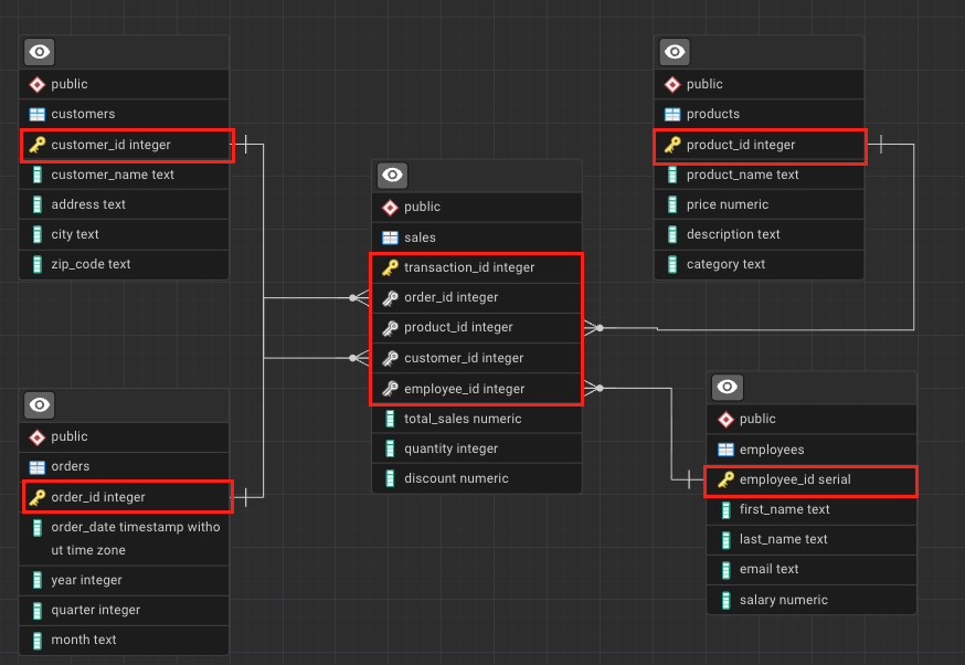
A relational database consists of one or more tables made up of rows and columns, and these tables are linked by relationships.

In this course, we will work with a sales analytics database that includes tables such as:

sales
orders
products
customers
employees

Each table stores information about a specific business entity, and relationships between tables allow us to combine this information during analysis.

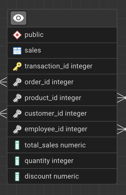
The list on the left represents all the columns in a table. Each column represents a specific attribute of a transaction, such as total_sales, quantity, or product_id. Each row (record) represents a single transaction.

Tip

Another name for a record is a tuple.

We will revisit tuples when working with Python and relational data.

Tables are such a common structure that you’ve likely interacted with them without realizing it.
For example, when you place an order on an e-commerce website like Amazon:

Each row represents a different order or transaction
Columns represent attributes such as:
- customer name
- address
- product ordered
- price
- order date

To illustrate, here’s an example order report.

Keys and Indexes

To store data efficiently and enable relationships between tables, relational databases rely on keys and indexes.

Keys

A key is a column (or set of columns) that uniquely identifies a row in a table.
Keys are essential for locating records and defining relationships between tables.

If you refer back to the sales table, you’ll notice a key icon next to the transaction_id column.
This indicates that transaction_id is a key.

In our database, each row in the sales table represents a single transaction line, uniquely identified by transaction_id.

Primary Key

A primary key uniquely identifies each record in a table.
Each table can have only one primary key, and it must:

Be unique
Never be NULL
Remain stable when referenced by other tables

In the sales table, transaction_id is the primary key.

transaction_id	order_id	product_id	customer_id	total_sales
1001	501	12	3001	49.99
1002	501	18	3001	19.99
1003	502	12	3005	49.99
1004	503	25	3008	89.99

Candidate Key

A candidate key is any column (or set of columns) that can uniquely identify a row.

For example, in the customers table, customer_id and email columns are candidate keys.

This means both columns are candidate keys.

From the set of candidate keys, one is chosen as the primary key.

In this schema, customer_id is selected as the primary key, while email remains an alternative identifier.

customer_id	customer_name	email	city
3001	Alice Johnson	alice.johnson@email.com	Berlin
3002	Mark Thompson	mark.thompson@email.com	Paris
3003	Elena Petrova	elena.p@email.com	Madrid
3004	David Chen	david.chen@email.com	London

Composite Key

A composite key is formed by combining two or more columns when no single column is sufficient to uniquely identify a row.

For example, (order_id, product_id) could uniquely identify rows in some transactional systems.

order_id	product_id	product_name	quantity
501	12	Wireless Mouse	1
501	18	USB-C Cable	2
502	12	Wireless Mouse	1
503	25	Mechanical Keyboard	1

In this table:

order_id alone is not unique
product_id alone is not unique
The combination (order_id, product_id) uniquely identifies each row

This combination forms a composite key.

Surrogate Key

A surrogate key is a system-generated identifier with no business meaning.

The transaction_id column is a surrogate key; its only purpose is to uniquely identify each transaction.

transaction_id	order_id	product_id	quantity	total_sales
1001	501	12	1	49.99
1002	501	18	2	19.99
1003	502	12	1	49.99
1004	503	25	1	89.99

Surrogate keys are often used even when natural or composite keys exist.

They are preferred in analytical systems because they:

simplify joins
reduce index size
improve query readability
remain stable even if business rules change

Foreign Key

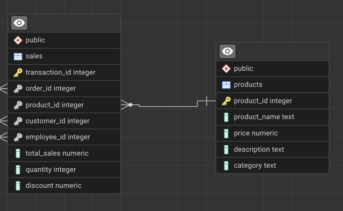
A foreign key is a column (or set of columns) that references a primary key in another table.

For example, the product_id column in the sales table references the product_id primary key in the products table.
Foreign keys establish relationships between tables and allow us to join data across entities.

Thus, Foreign key enforces referential integrity between the two tables which is crucial:

prevent invalid data (e.g., sales for non-existent products)
define how tables are related
enable joins between tables
preserve data consistency

Important

In analytical databases, foreign keys are sometimes not physically enforced for performance reasons, but they are always enforced logically in the data model.

Indexes

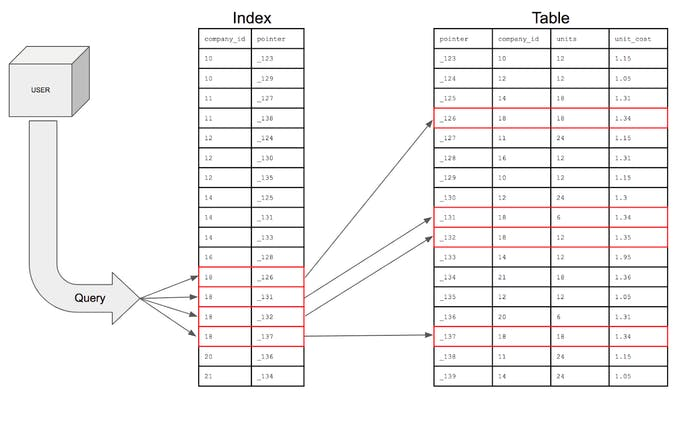
Imagine searching through a book to find all pages starting with the letter A.
Without an index, you would scan every page.
With an index (like a dictionary), you jump directly to the correct section.

Indexes work the same way in databases.

Indexes do not store new data.
They are special lookup structures that improve query performance.

Full Table Scan

When a query checks every row instead of using an index, this is called a full scan.

Indexes improve read performance but come with trade-offs:

extra storage
slower inserts and updates
maintenance overhead

When Not to Create Indexes

Very small tables
Frequently updated columns
Columns with many NULL values
Columns with very low cardinality

Single-Column Index

A single-column index is built on one column.

Employee ID	Name	Contact Number	Age
1	Max	800692692	24
2	Jessica	800123456	35
3	Mikeal	800745547	49

Composite Index

Consider the same employees table, but now imagine that queries often filter by both name and age at the same time. Thus, composite index spans multiple columns, such as (name, age).

Composite indexes are most effective when queries filter columns in the same left-to-right order as the index definition.

employee_id	name	age	department
1	Max	24	Sales
2	Jessica	35	Marketing
3	Max	35	Finance

For an index defined as (name, age):

Efficient for queries filtering on name
Efficient for queries filtering on name and age
Not efficient for queries filtering on age only

Unique Index

Unlike a regular index, a unique index enforces a rule, not just performance. A unique index ensures that values are not duplicated.

customer_id	customer_name	email
3001	Alice Johnson	alice@email.com
3002	Mark Thompson	mark@email.com
3003	Elena Petrova	elena@email.com

In the aboive table:

email values are unique
No two customers share the same email address

Creating a unique index on email:

prevents duplicate emails
guarantees data integrity

Use a unique index when:

values must be unique across rows
the column is frequently used for lookup
uniqueness is part of business logic

Are Keys Also Indexes?

Keys vs Indexes

From a database engine and storage point of view, keys and indexes are closely related, but they are not the same thing.

A key defines a logical rule (uniqueness, relationships)
An index is a physical data structure stored on disk to speed up access

How PostgreSQL Handles Them

Concept	Enforces Uniqueness	Improves Query Speed	Stored as Index
Primary Key	Yes	Yes	Yes (unique index)
Unique Constraint	Yes	Yes	Yes (unique index)
Foreign Key	No	Sometimes	No (by default)
Regular Index	No	Yes	Yes

Important Notes

Creating a primary key automatically creates a unique index
Creating a unique constraint automatically creates a unique index
Foreign keys do NOT create indexes automatically
Indexes exist to improve performance; keys exist to enforce rules

Data Types

Data types define what kind of data a column can store.
They ensure consistency, enable validation, and affect performance.

Consider the following example:

Employee Name	Salary ($)
Jan	100000
Alex	One hundred thousand
Kim	70k

Caution

Inconsistent data types make analysis impossible.

To calculate averages or totals, the column must enforce a numeric type.

Data Types in PostgreSQL

Numeric
Character
Date & Time
Boolean & Categorical
Identifier & Auto-Increment
JSON and Semi-Structured
Array
Special Data Types

Numeric Data Types

In PostgreSQL, numeric data types fall into three main groups:

Integers: whole numbers
Exact numerics: precise decimal numbers
Floating-point numbers: approximate decimals

Numeric data types are used for:

counts
quantities
prices
measurements

Main Numeric Data Types

Data Type	Description	Example Value	Memory Size	Typical Use Case
SMALLINT	Small-range whole numbers	12	2 bytes	Status codes, flags
INTEGER / INT	Standard whole numbers	2500	4 bytes	Quantities, counts
BIGINT	Very large whole numbers	9876543210	8 bytes	IDs, large counters
NUMERIC(p, s)	Exact precision decimal	NUMERIC(10,2) → 15432.75	Variable	Salary, revenue
DECIMAL(p, s)	Same as NUMERIC (SQL standard)	DECIMAL(8,3) → 123.456	Variable	Financial data
REAL	Approximate floating-point	3.14159	4 bytes	Scientific values
DOUBLE PRECISION	Higher-precision floating-point	0.0000123456789	8 bytes	Statistical calculations

Note

Notice how exact numerics (NUMERIC, DECIMAL) preserve precision, while floating-point types (REAL, DOUBLE PRECISION) may introduce rounding differences.

Performance vs Precision Trade-off

When choosing a numeric data type, you must balance precision, performance, and storage efficiency.
The table below summarizes the most common analytical requirements and the recommended PostgreSQL data types.

Requirement	Precision Needed	Performance Priority	Recommended Data Type
Row counts, simple counters	Exact	Very high	INTEGER
Large identifiers (IDs)	Exact	High	BIGINT
Financial values (salary, revenue)	Exact	Medium	NUMERIC(p,s)
Prices with decimals	Exact	Medium	DECIMAL(p,s)
Ratios, averages, KPIs	Approximate acceptable	High	DOUBLE PRECISION
Scientific measurements	Approximate acceptable	Very high	REAL / DOUBLE PRECISION

Index Size Considerations

Indexes inherit the storage and performance characteristics of the column type they are built on:

Index on INTEGER $\rightarrow$ small $\rightarrow$ cache-friendly
Index on NUMERIC $\rightarrow$ larger $\rightarrow$ slower to scan
Composite indexes amplify the effect of column size

Best Practice

Use the smallest numeric type that safely fits your data.

Prefer INTEGER over BIGINT if values fit
Use NUMERIC only when precision matters
Avoid premature use of NUMERIC for IDs or counters

Character Data Types

Character data types are used to store textual information such as names, descriptions, identifiers, and free-form text.

In PostgreSQL, character data types fall into three main groups:

Fixed-length characters — text with a fixed size
Variable-length characters — text with flexible size limits
Unbounded text — long or unpredictable text

Character data types are used for:

names
descriptions
emails
codes
comments

Main Character Data Types

Data Type	Description	Example Value	Memory Size	Typical Use Case
CHAR(n)	Fixed-length character string	CHAR(5) → ‘US’	n bytes (fixed)	Country codes, fixed formats
VARCHAR(n)	Variable-length string with limit	VARCHAR(50) → ‘Karen Hovhannisyan’	Variable (≤ n)	Names, emails
TEXT	Variable-length string, no limit	‘This product has been discontinued.’	Variable	Descriptions, comments
CHARACTER VARYING(n)	SQL-standard name for VARCHAR	CHARACTER VARYING(20) → ‘A123XZ’	Variable (≤ n)	Codes, identifiers

Note

VARCHAR(n) and TEXT behave almost identically in PostgreSQL.
The main difference is whether you want to enforce a maximum length.

Performance vs Flexibility Trade-off

When choosing a character data type, the trade-off is usually between data validation and flexibility, not raw performance.

Requirement	Length Control Needed	Flexibility Priority	Recommended Data Type
Fixed-format values	Yes (fixed)	Low	CHAR(n)
Names, emails	Yes (reasonable limit)	Medium	VARCHAR(n)
Free-form text	No	High	TEXT
User comments, notes	No	Very high	TEXT

Index Size Considerations

Indexes on character columns depend on string length and value distribution:

Index on CHAR(n) $\rightarrow$ predictable size $\rightarrow$ stable performance
Index on VARCHAR(n) $\rightarrow$ variable size $\rightarrow$ generally efficient
Index on TEXT $\rightarrow$ potentially large $\rightarrow$ slower scans for long values
Long strings in composite indexes increase index size significantly

Best Practice

Use constraints, not oversized text types, to control data quality.

Prefer VARCHAR(n) when a reasonable maximum length exists
Use TEXT for descriptions and comments
Avoid CHAR(n) unless values are truly fixed-length

Date & Time Data Types

Date and time data types are used to store temporal information, such as when an event occurred, started, or ended.

They are critical for analytics involving time series, trends, seasonality, and durations.

In PostgreSQL, date and time data types fall into four main groups:

Date-only values
Time-only values
Timestamps (date + time)
Time intervals / durations

Date & time data types are used for:

event dates
timestamps
log records
durations
time-based analysis

Main Date & Time Data Types

Data Type	Description	Example Value	Memory Size	Typical Use Case
DATE	Calendar date (no time)	2025-03-15	4 bytes	Birth dates, order dates
TIME	Time of day (no date)	14:30:00	8 bytes	Opening hours
TIME WITH TIME ZONE	Time with time zone info	14:30:00+04	12 bytes	Cross-region schedules
TIMESTAMP	Date and time (no timezone)	2025-03-15 14:30:00	8 bytes	Local event logs
TIMESTAMP WITH TIME ZONE (TIMESTAMPTZ)	Date and time with timezone handling	2025-03-15 10:30:00+00	8 bytes	Auditing, analytics
INTERVAL	Time duration	3 days 4 hours	16 bytes	Session length, SLA

Note

TIMESTAMPTZ does not store the time zone itself.
PostgreSQL converts values to UTC internally and displays them using the session time zone.

Accuracy vs Interpretability Trade-off

When working with time data, the trade-off is often between absolute correctness and human interpretation.

Requirement	Time Zone Awareness	Recommended Data Type
Simple dates	Not needed	DATE
Local business timestamps	Not required	TIMESTAMP
Multi-region systems	Required	TIMESTAMPTZ
Durations and differences	Not applicable	INTERVAL

Index Size Considerations

Date and time types are fixed-size, making them efficient for indexing:

Index on DATE $\rightarrow$ small $\rightarrow$ very fast range scans
Index on TIMESTAMP $\rightarrow$ small $\rightarrow$ efficient sorting
Index on TIMESTAMPTZ $\rightarrow$ small $\rightarrow$ timezone-safe
Index on INTERVAL $\rightarrow$ rarely indexed (use carefully)

Date-based indexes are commonly used with:

WHERE date BETWEEN …
GROUP BY date
time-window queries

Best Practice

Always use TIMESTAMPTZ for analytics and logging systems.

Avoid ambiguity in multi-region environments
Use DATE only when time is irrelevant
Store durations as INTERVAL, not numeric hacks

Boolean & Categorical Data Types

Boolean and categorical data types are used to store logical values and finite categories.
They are especially important for filtering, segmentation, and business rules.

In PostgreSQL, boolean and categorical data types fall into two main groups:

Boolean values — true / false logic
Categorical values — limited sets of labels

These data types are used for:

flags
status indicators
binary decisions
categorical segmentation

Main Boolean & Categorical Data Types

Data Type	Description	Example Value	Memory Size	Typical Use Case
BOOLEAN	Logical true / false value	TRUE, FALSE	1 byte	Active flags, eligibility
CHAR(n)	Fixed-length category code	CHAR(1) → ‘Y’	n bytes (fixed)	Yes/No indicators
VARCHAR(n)	Short categorical label	‘premium’	Variable (≤ n)	Customer segments
TEXT	Free-form category label	‘high_value_customer’	Variable	Tags, labels
ENUM	Predefined set of values	(‘low’,‘medium’,‘high’)	4 bytes	Controlled categories

Caution

PostgreSQL accepts multiple boolean literals:

TRUE / FALSE, true / false, 1 / 0, yes / no.

Control vs Flexibility Trade-off

The main trade-off for categorical data is between data integrity and flexibility.

Requirement	Validation Strictness	Recommended Data Type
Binary logic	Very strict	BOOLEAN
Small fixed category set	Very strict	ENUM
Evolving categories	Medium	VARCHAR(n)
User-defined labels	Low	TEXT

Index Size Considerations

Index on BOOLEAN $\rightarrow$ very small $\rightarrow$ fast but often low selectivity
Index on short categorical strings $\rightarrow$ efficient
Index on high-cardinality categories $\rightarrow$ more useful than boolean indexes
Avoid indexing columns with very few distinct values

Best Practice

Use BOOLEAN only for true binary logic.

Do not encode booleans as ‘Y’/‘N’ unless required
Use ENUM only when categories are stable

Special & Advanced Data Types | OPTIONAL

Beyond standard numeric, text, and date types, PostgreSQL supports specialized data types designed for specific domains such as

geospatial analysis
networks
graphsand
semi-structured data.

These data types are typically used in advanced analytics, telecom, log analysis, and platform-scale systems.

Special data types are used for:

geospatial analytics
network analysis
semi-structured data
system-level identifiers
advanced domain modeling

Main Special Data Types (with Example Values)

Data Type / Extension	Description	Example Value	Typical Use Case
JSON / JSONB	Semi-structured JSON data	{“plan”:“premium”,“usage”:120}	Logs, APIs, configs
ARRAY	Array of values	{1,2,3}	Tags, multi-valued attributes
UUID	Universally unique identifier	550e8400-e29b-41d4-a716-446655440000	Distributed IDs
INET	IP address	192.168.1.1	Network traffic
CIDR	Network block	192.168.0.0/24	Subnet modeling
GEOMETRY (PostGIS)	Geometric objects	POINT(40.18 44.51)	Maps, locations
GEOGRAPHY (PostGIS)	Earth-based coordinates	POINT(44.51 40.18)	Distance calculations
ltree	Hierarchical tree paths	region.city.store	Organizational trees
pgRouting	Graph/network extension	N/A	Network routing, telecom

Note

Most advanced data types are provided via PostgreSQL extensions, not core SQL.

Domain-Specific Trade-offs

Special data types trade generality for domain power.

Requirement	Domain	Recommended Type
Flexible event payloads	Logging / APIs	JSONB
Multi-valued attributes	Analytics	ARRAY
Globally unique IDs	Distributed systems	UUID
IP & network data	Telecom / IT	INET, CIDR
Location-based analytics	GIS	PostGIS (GEOMETRY / GEOGRAPHY)
Graph traversal	Networks	pgRouting, graph models

Indexing & Performance Considerations

Special data types usually require specialized indexes:

JSONB $\rightarrow$ GIN index
GEOMETRY / GEOGRAPHY $\rightarrow$ GiST / SP-GiST
ARRAY $\rightarrow$ GIN
INET / CIDR $\rightarrow$ GiST

Improper indexing can make these types very slow on large datasets.

Performance Warning

Advanced data types without proper indexes often lead to full scans, even on indexed tables.

PostGIS (Geospatial Extension)

PostGIS adds geospatial intelligence to PostgreSQL.

Common capabilities:

Distance calculations
Spatial joins
Radius searches
Area coverage

Important

As a data analyst you are not expected to design PostGIS schemas or routing graphs — but you will query them.

Data Dictionary

A data dictionary documents metadata such as:

table names
column descriptions
keys and constraints
relationships

As an analyst, the data dictionary helps you understand where data lives and how to query it correctly.

Overview

This data dictionary describes the structure and meaning of the tables used in the sales analytics database.

table purpose
column definitions
data types
keys and relationships

Table: `employees`

Description
Stores information about employees involved in the sales process.

Column Name	Data Type	Key	Description
`employee_id`	`SERIAL`	PK	Unique identifier for each employee
`first_name`	`TEXT`		Employee first name
`last_name`	`TEXT`		Employee last name
`email`	`TEXT`		Employee email address
`salary`	`NUMERIC`		Employee salary

Table: `customers`

Description
Stores customer profile and location information.

Column Name	Data Type	Key	Description
`customer_id`	`INTEGER`	PK	Unique identifier for each customer
`customer_name`	`TEXT`		Full customer name
`address`	`TEXT`		Customer address
`city`	`TEXT`		City of residence
`zip_code`	`TEXT`		Postal / ZIP code

Table: `products`

Description
Contains product catalog information.

Column Name	Data Type	Key	Description
`product_id`	`INTEGER`	PK	Unique product identifier
`product_name`	`TEXT`		Name of the product
`price`	`NUMERIC`		Unit price of the product
`description`	`TEXT`		Product description
`category`	`TEXT`		Product category

Table: `orders`

Description
Stores order-level information and time attributes.

Column Name	Data Type	Key	Description
`order_id`	`INTEGER`	PK	Unique order identifier
`order_date`	`TIMESTAMP`		Date and time when the order was placed
`year`	`INTEGER`		Order year (derived)
`quarter`	`INTEGER`		Order quarter (derived)
`month`	`TEXT`		Order month name (derived)

Table: `sales`

Description
Central fact table storing individual sales transaction lines.

Column Name	Data Type	Key	Description
`transaction_id`	`INTEGER`	PK	Unique transaction identifier (surrogate key)
`order_id`	`INTEGER`	FK	References `orders(order_id)`
`product_id`	`INTEGER`	FK	References `products(product_id)`
`customer_id`	`INTEGER`	FK	References `customers(customer_id)`
`employee_id`	`INTEGER`	FK	References `employees(employee_id)`
`total_sales`	`NUMERIC`		Total sales value for the transaction
`quantity`	`INTEGER`		Number of units sold
`discount`	`NUMERIC`		Discount applied to the transaction

Relationships Summary

From Table	Column	To Table	Column	Relationship Type
`sales`	`order_id`	`orders`	`order_id`	Many-to-one
`sales`	`product_id`	`products`	`product_id`	Many-to-one
`sales`	`customer_id`	`customers`	`customer_id`	Many-to-one
`sales`	`employee_id`	`employees`	`employee_id`	Many-to-one

Analyst Notes

sales is the fact table
Other tables act as dimensions
transaction_id is a surrogate key
Time attributes are intentionally denormalized
Foreign keys may be logically enforced in analytical systems

DDL: Data Definition Language

DDL (Data Definition Language) is responsible for defining and managing the structure of a database.

DDL statements operate on database objects, not on individual rows.
They describe what the database looks like, not what data it contains.

DDL is foundational: every data operation you perform later depends on decisions made at the DDL level.

Common DDL Statements

DDL includes the following core commands:

CREATE
ALTER
DROP
TRUNCATE

Each of these affects database schema and metadata.

CREATE (DDL Context)

In the context of DDL, CREATE is used to define new database objects, such as tables and indexes.

Typical use cases include:

creating analytical tables
creating staging tables
creating indexes to improve performance

Example: create an index to support analytical queries.

CREATE INDEX idx_sales_product_id
ON sales (product_id);

This command does not modify data.
It changes how efficiently the database can access existing data.

ALTER

The ALTER statement modifies the structure of an existing database object.

Common use cases include:

adding columns
enforcing constraints
changing column properties

ALTER TABLE products
ADD CONSTRAINT chk_products_price
CHECK (price >= 0);

DROP

The DROP statement permanently removes a database object.

DROP INDEX idx_sales_product_id;

DROP TABLE products;

This operation is irreversible and should be used with extreme caution.

TRUNCATE

TRUNCATE removes all rows from a table while keeping its structure intact.

TRUNCATE TABLE sales_staging;

CRUD: Data Manipulation in Practice

CRUD describes how we work with data inside existing tables.
These are the SQL operations data analysts use most frequently.

CRUD stands for:

CREATE
READ
UPDATE
DELETE

Critical Terminology Clarification

The word CREATE means different things in different contexts.

DDL CREATE $\rightarrow$ creates database objects (tables, indexes)
CRUD CREATE $\rightarrow$ inserts new data (INSERT)

Confusing these two is one of the most common beginner mistakes.

DDL vs CRUD — Conceptual Comparison

DDL $\rightarrow$ defines the structure
CRUD $\rightarrow$ manipulates the data
DDL $\rightarrow$ happens rarely
CRUD $\rightarrow$ happens constantly

DDL sets the rules.
CRUD must follow them.

CREATE (CRUD $\rightarrow$ INSERT)

In the CRUD context, CREATE means adding new rows to an existing table.

This is done using the INSERT statement.

INSERT INTO products (product_id, product_name, price, category)
VALUES (101, 'Wireless Mouse', 24.99, 'Accessories');

You may omit columns that allow NULL or have default values.

INSERT INTO products (product_id, product_name, price)
VALUES (102, 'USB-C Cable', 9.99);

READ (SELECT)

The READ operation retrieves data and is implemented using SELECT.

SELECT
  product_id,
  product_name
FROM products;

Filtering rows is done using WHERE.

SELECT
  *
FROM sales
WHERE total_sales < 50;

UPDATE

The UPDATE statement modifies existing records.

Updates should always target specific rows.

UPDATE products
SET price = 49.99
WHERE product_id = 12;

DELETE

The DELETE statement removes records from a table.

Because deletions are irreversible, this command must be used with extreme caution.

DELETE FROM sales
WHERE transaction_id = 1004;

Mental Model to Remember

DDL $\rightarrow$ defines tables, columns, constraints, indexes
CRUD $\rightarrow$ inserts, reads, updates, deletes rows
DML $\rightarrow$ SQL language (INSERT, SELECT, UPDATE, DELETE) implementing CRUD

The first part of DML will be introduced in Session 3.
You can revisit it here: Session 3 DML Basics

To Quote or Not to Quote?

When writing SQL statements, make sure to place quotes around non-numeric values such as text and dates.

For example, in an INSERT command:

text values like title and description must be enclosed in quotes
numeric values like language_id and release_year should not

Different database systems handle quotes differently.

PostgreSQL accepts single quotes only (’’) for string literals, while some other systems allow both single and double quotes.

Constraints

I used the constraints above the lecture note, and decided to do a deep dive here as well :)

In this section, you’ll be looking at constraints, which play a crucial role in keeping your data organized.

Constraints specify what type of data a table or column can accept, and they are typically set when a table is created. When defined correctly, constraints:

enforce data integrity
prevent invalid or inconsistent data
act as built-in data quality checks

Below are the most common constraints you will encounter when designing relational databases.

UNIQUE Constraint

The UNIQUE constraint ensures that all values in a column are distinct.
It is commonly used to prevent duplicate records for attributes that must be unique across entities.

Typical use cases include:

email addresses
usernames
national identification numbers

Example: ensure each customer email is unique.

CREATE TABLE customers (
  customer_id INTEGER PRIMARY KEY,
  email TEXT UNIQUE,
  phone_number TEXT
);

With this constraint in place, PostgreSQL will reject any attempt to insert a duplicate email address.

NOT NULL Constraint

The NOT NULL constraint ensures that a column cannot contain empty (NULL) values.

Use this constraint for fields that are mandatory and must always be provided.

Typical use cases include:

primary identifiers
contact information
transaction timestamps

Example: ensure every customer has a phone number.

CREATE TABLE customers (
  customer_id INTEGER PRIMARY KEY,
  phone_number TEXT NOT NULL,
  email TEXT
);

If an insert is attempted without a phone number, PostgreSQL will return an error.

PRIMARY KEY Constraint

A PRIMARY KEY uniquely identifies each row in a table.

A primary key:

must be unique
cannot contain NULL values
exists only once per table

Example: define a primary key for a products table.

CREATE TABLE products (
  product_id INTEGER PRIMARY KEY,
  product_name TEXT NOT NULL,
  price NUMERIC(10, 2)
);

The PRIMARY KEY constraint automatically enforces both UNIQUE and NOT NULL.

FOREIGN KEY Constraint

A FOREIGN KEY creates a relationship between two tables by referencing the primary key of another table.

It ensures referential integrity, meaning that referenced values must exist in the parent table.

Example: link sales records to customers.

CREATE TABLE sales (
  transaction_id INTEGER PRIMARY KEY,
  customer_id INTEGER,
  total_sales NUMERIC(10, 2),
  FOREIGN KEY (customer_id)
    REFERENCES customers (customer_id)
);

With this constraint, you cannot insert a sale for a customer that does not exist in the customers table.

CHECK Constraint

The CHECK constraint restricts the range or condition of values that can be inserted into a column.

It validates data based on logical expressions.

Typical use cases include:

value ranges
minimum or maximum limits
domain rules

Example: ensure total sales values are non-negative.

CREATE TABLE sales (
  transaction_id INTEGER PRIMARY KEY,
  total_sales NUMERIC(10, 2) CHECK (total_sales >= 0)
);

If a value violates the condition, the insert or update will fail with an error.

SQL Rules and Best Practices

Now that you’ve seen the most common SQL statements, let’s get to grips with some basic rules and best practices for using SQL.
This list is not exhaustive—it is a starting point. As you gain hands-on experience, you will naturally pick up additional techniques and conventions.

Numbers and Underscores

In a relational database:

Table names and column names cannot start with a number
They cannot contain spaces
Use underscores (_) to separate words

This improves compatibility and readability.

Recommended

CREATE TABLE customer_lifecycle;
CREATE TABLE customer;

Not Recommended

CREATE TABLE customer lifecycle;
CREATE TABLE 3customer;

Capitalization

A widely accepted convention is:

SQL keywords → UPPERCASE
Table names → lowercase
Column names → lowercase

This makes queries easier to scan and understand.

Recommended

SELECT product_id, product_name
FROM products;

SELECT transaction_id, total_sales
FROM sales;

Not Recommended

Select PRODUCT_ID, PRODUCT_NAME From PRODUCTS;

SELECT TRANSACTION_ID, TOTAL_SALES FROM SALES;

Commenting

It is good practice to comment your SQL code so that other analysts and developers can easily read and understand your queries.

Comments do not affect query execution—they exist purely for documentation and readability.

Use -- for single-line comments.

-- select and display the first 10 rows from the sales table
SELECT *
FROM sales
LIMIT 10;

Multi-line comments can also be used to temporarily disable blocks of SQL code during testing or debugging.

/*
SELECT
  s.transaction_id,
  p.product_name,
  s.total_sales
FROM sales s
JOIN products p
  ON s.product_id = p.product_id
WHERE s.total_sales > 100;
*/

Aliasing

Aliases assign temporary names to columns or tables within a query.

They are especially useful for:

improving readability
shortening long names
resolving ambiguity in joins

Column aliases rename columns in the query output.

SELECT
  product_name AS item_name,
  price AS unit_price
FROM products;

Table aliases are commonly used in joins.

SELECT
  s.transaction_id,
  p.product_name,
  s.total_sales
FROM sales AS s
JOIN products AS p
  ON s.product_id = p.product_id;

Tip

Here you will find much more tips

Sales Analytics Database

Learning Goals

Data Storage Structures

Keys and Indexes

Keys

Primary Key

Candidate Key

Composite Key

Surrogate Key

Foreign Key

Indexes

When Not to Create Indexes

Single-Column Index

Composite Index

Unique Index

Keys vs Indexes

How PostgreSQL Handles Them

Important Notes

Data Types

Data Types in PostgreSQL

Numeric Data Types

Main Numeric Data Types

Performance vs Precision Trade-off

Index Size Considerations

Character Data Types

Main Character Data Types

Performance vs Flexibility Trade-off

Index Size Considerations

Date & Time Data Types

Main Date & Time Data Types

Accuracy vs Interpretability Trade-off

Index Size Considerations

Boolean & Categorical Data Types

Main Boolean & Categorical Data Types

Control vs Flexibility Trade-off

Index Size Considerations

Special & Advanced Data Types | OPTIONAL

Main Special Data Types (with Example Values)

Domain-Specific Trade-offs

Indexing & Performance Considerations

PostGIS (Geospatial Extension)

Data Dictionary

Overview

Table: employees

Table: customers

Table: products

Table: orders

Table: sales

Relationships Summary

Analyst Notes

DDL: Data Definition Language

Common DDL Statements

CREATE (DDL Context)

ALTER

DROP

TRUNCATE

CRUD: Data Manipulation in Practice

CREATE (CRUD \(\rightarrow\) INSERT)

READ (SELECT)

UPDATE

DELETE

Constraints

UNIQUE Constraint

NOT NULL Constraint

PRIMARY KEY Constraint

FOREIGN KEY Constraint

CHECK Constraint

SQL Rules and Best Practices

Numbers and Underscores

Capitalization

Commenting

Aliasing

Table: `employees`

Table: `customers`

Table: `products`

Table: `orders`

Table: `sales`