Advanced SQL Functions
Window Functions
2026-07-04
Transition to Window Functions
CTEs define what is computed and in what order.
Window Functions define how rows are compared.
Window Functions
Core Idea (Syntax Skeleton)
Window Functions vs Aggregations
| Feature | GROUP BY | Window Function |
|---|---|---|
| Rows preserved | No | Yes |
| Aggregation scope | Entire group | Sliding / contextual |
| Output rows | Fewer | Same as input |
| Analytical use | Summaries | Comparisons, trends |
Simple Conceptual Example
Input Table: sales
| order_id | customer_id | order_date | revenue |
|---|---|---|---|
| 1 | 10 | 2024-01-01 | 100 |
| 2 | 10 | 2024-01-05 | 150 |
| 3 | 20 | 2024-01-03 | 200 |
Question: Show each order and the total revenue per customer.
| order_id | customer_id | revenue | total_customer_revenue |
|---|---|---|---|
| 1 | 10 | 100 | 250 |
| 2 | 10 | 150 | 250 |
| 3 | 20 | 200 | 200 |
Analytical Value of Window Functions
- Comparing rows to group averages
- Ranking and ordering observations
- Measuring change over time
- Calculating running totals
- Detecting trends and anomalies
Window Functions in Data Aalytics
- Customer lifetime analysis
- Time-series trend comparison
- Cohort analysis
- Funnel progression
- Ranking and segmentation
Window functions are a cornerstone of modern analytical SQL.
| Construct | Purpose |
|---|---|
| Temporary Tables | Reuse intermediate results |
| Subqueries | Inline conditions and metrics |
| Derived Tables | Inline datasets |
| CTEs | Named pipelines |
| Window Functions | Context-aware row analytics |
Temporary Table
CREATE TEMP TABLE tmp_sales AS
SELECT *
FROM (
    VALUES

        (1,  'A', DATE '2024-01-01', 100, 'online'),
        (2,  'A', DATE '2024-01-02', 120, 'store'),
        (3,  'A', DATE '2024-01-03', 90,  'online'),
        (4,  'A', DATE '2024-01-04', 130, 'store'),


        (5,  'B', DATE '2024-01-01', 180, 'store'),
        (6,  'B', DATE '2024-01-02', 200, 'online'),
        (7,  'B', DATE '2024-01-03', 220, 'online'),
        (8,  'B', DATE '2024-01-04', 200, 'store'),


        (9,  'C', DATE '2024-01-01', 150, 'online'),
        (10, 'C', DATE '2024-01-02', 150, 'online'),
        (11, 'C', DATE '2024-01-03', 170, 'online'),


        (12, 'D', DATE '2024-01-01', 90,  'store'),
        (13, 'D', DATE '2024-01-02', 110, 'store'),


        (14, 'E', DATE '2024-01-01', 140, 'store'),
        (15, 'E', DATE '2024-01-02', 160, 'online'),
        (16, 'E', DATE '2024-01-03', 155, 'store')
) AS t(
    sale_id,
    customer_id,
    sale_date,
    amount,
    channel
);
Window Function Layers
- Aggregate over a window (e.g.,
SUM(),AVG(),COUNT())
- Navigational & Value from another row (e.g.,
LAG(),LEAD(),FIRST_VALUE(),LAST_VALUE())
- Ranking functions (e.g.,
ROW_NUMBER(),RANK(),DENSE_RANK())
- Cumulative distributions (e.g.,
CUME_DIST(),PERCENT_RANK())
- String aggregation (e.g.,
STRING_AGG()) - Framing & Advanced Window Control (Advanced)
Simple Aggregate Window Functions
Concept
Simple aggregate window functions apply classical aggregation logic (such as SUM, AVG, COUNT, MIN, MAX) without collapsing rows.
They answer the question:
How does this row relate to an aggregate of its group/partition?
Common Functions in This Layer
SUM()
AVG()
COUNT()
MIN()
MAX()
All of them become window functions when combined with OVER(...).
Example: Average Amount per Customer
Business intuition: “How much does this sale differ from the customer’s typical behavior?”
| sale_id | customer_id | amount | avg_customer_amount |
|---|---|---|---|
| 1 | A | 100 | 110.00 |
| 2 | A | 120 | 110.00 |
| 5 | B | 200 | 200.00 |
| 6 | B | 180 | 200.00 |
| 7 | B | 220 | 200.00 |
| 8 | B | 200 | 200.00 |
| 10 | C | 150 | 156.67 |
| 11 | C | 170 | 156.67 |
Statistical Window Functions
Concept
Statistical window functions extend simple aggregates by answering distributional questions instead of basic totals or averages.
They answer the question:
Where does this row stand within the distribution of its group?
Common Functions in This Layer
PERCENTILE_CONT()
PERCENTILE_DISC()
PERCENT_RANK()
CUME_DIST()
Generic Pattern
Example 1: PERCENTILE_CONT() of Sale Amount
Business intuition: “What is the typical (middle) transaction size for this customer?”
| customer_id | median_amount |
|---|---|
| B | 200 |
| C | 150 |
| D | 100 |
| E | 155 |
Example 2: Percent Rank of Each Transaction
PERCENT_RANK() shows relative position between 0 and 1.
| sale_id | customer_id | amount | percent_rank |
|---|---|---|---|
| 3 | A | 90 | 0.000 |
| 1 | A | 100 | 0.333 |
| 2 | A | 120 | 0.667 |
| 4 | A | 130 | 1.000 |
| 5 | B | 180 | 0.000 |
| 6 | B | 200 | 0.333 |
| 8 | B | 200 | 0.333 |
| 7 | B | 220 | 1.000 |
| 9 | C | 150 | 0.000 |
| 10 | C | 150 | 0.000 |
| 11 | C | 170 | 1.000 |
| 12 | D | 90 | 0.000 |
| 13 | D | 110 | 1.000 |
| 14 | E | 140 | 0.000 |
| 16 | E | 155 | 0.500 |
| 15 | E | 160 | 1.000 |
Example 3: Cumulative Distribution
CUME_DIST() shows the share of rows less than or equal to the current row.
| sale_id | customer_id | amount | cumulative_distribution |
|---|---|---|---|
| 3 | A | 90 | 0.25 |
| 1 | A | 100 | 0.5 |
| 2 | A | 120 | 0.75 |
| 4 | A | 130 | 1 |
| 5 | B | 180 | 0.25 |
| 6 | B | 200 | 0.75 |
| 8 | B | 200 | 0.75 |
| 7 | B | 220 | 1 |
| 9 | C | 150 | 0.666 |
| 10 | C | 150 | 0.666 |
| 11 | C | 170 | 1 |
| 12 | D | 90 | 0.5 |
| 13 | D | 110 | 1 |
| 14 | E | 140 | 0.333 |
| 16 | E | 155 | 0.666 |
| 15 | E | 160 | 1 |
Important
- Statistical window functions are order-sensitive
- They expose distribution shape
- Results are relative, not absolute
- They are critical for:
- Outlier detection
- Segmentation
- Threshold-based decisions
- Outlier detection
Value from Another Row Functions
Concept
How does this row relate to previous or next rows in sequence?
Value-from-another-row functions enable row-to-row comparisons within a defined order, facilitating trend analysis and change detection.
Tip
These functions are inherently time-aware and sequence-aware.
Generic Pattern
offset(optional) defines how many rows forward/backward to look- Default offset is
1
Example 1: Previous Transaction Amount (LAG)
Business intuition:
“How did this transaction change compared to the previous one?”
| sale_id | customer_id | sale_date | amount | previous_amount |
|---|---|---|---|---|
| 1 | A | 2024-01-01 | 100 | |
| 2 | A | 2024-01-02 | 120 | 100 |
| 3 | A | 2024-01-03 | 90 | 120 |
| 4 | A | 2024-01-04 | 130 | 90 |
| 5 | B | 2024-01-01 | 180 | |
| 6 | B | 2024-01-02 | 200 | 180 |
| 7 | B | 2024-01-03 | 220 | 200 |
| 8 | B | 2024-01-04 | 200 | 220 |
| 9 | C | 2024-01-01 | 150 | |
| 10 | C | 2024-01-02 | 150 | 150 |
| 11 | C | 2024-01-03 | 170 | 150 |
| 12 | D | 2024-01-01 | 90 | |
| 13 | D | 2024-01-02 | 110 | 90 |
| 14 | E | 2024-01-01 | 140 | |
| 15 | E | 2024-01-02 | 160 | 140 |
| 16 | E | 2024-01-03 | 155 | 160 |
Example 2: Next Transaction Amount (LEAD)
| sale_id | customer_id | sale_date | amount | next_amount |
|---|---|---|---|---|
| 1 | A | 2024-01-01 | 100 | 120 |
| 2 | A | 2024-01-02 | 120 | 90 |
| 3 | A | 2024-01-03 | 90 | 130 |
| 4 | A | 2024-01-04 | 130 | |
| 5 | B | 2024-01-01 | 180 | 200 |
| 6 | B | 2024-01-02 | 200 | 220 |
| 7 | B | 2024-01-03 | 220 | 200 |
| 8 | B | 2024-01-04 | 200 | |
| 9 | C | 2024-01-01 | 150 | 150 |
| 10 | C | 2024-01-02 | 150 | 170 |
| 11 | C | 2024-01-03 | 170 | |
| 12 | D | 2024-01-01 | 90 | 110 |
| 13 | D | 2024-01-02 | 110 | |
| 14 | E | 2024-01-01 | 140 | 160 |
| 15 | E | 2024-01-02 | 160 | 155 |
| 16 | E | 2024-01-03 | 155 |
Example 3: First Transaction Amount per Customer
| sale_id | customer_id | sale_date | amount | first_amount |
|---|---|---|---|---|
| 1 | A | 2024-01-01 | 100 | 100 |
| 2 | A | 2024-01-02 | 120 | 100 |
| 3 | A | 2024-01-03 | 90 | 100 |
| 4 | A | 2024-01-04 | 130 | 100 |
| 5 | B | 2024-01-01 | 180 | 180 |
| 6 | B | 2024-01-02 | 200 | 180 |
| 7 | B | 2024-01-03 | 220 | 180 |
| 8 | B | 2024-01-04 | 200 | 180 |
| 9 | C | 2024-01-01 | 150 | 150 |
| 10 | C | 2024-01-02 | 150 | 150 |
| 11 | C | 2024-01-03 | 170 | 150 |
| 12 | D | 2024-01-01 | 90 | 90 |
| 13 | D | 2024-01-02 | 110 | 90 |
| 14 | E | 2024-01-01 | 140 | 140 |
| 15 | E | 2024-01-02 | 160 | 140 |
| 16 | E | 2024-01-03 | 155 | 140 |
Ranking Functions
Concept
They answer the question:
How does this row rank relative to other rows in its group?
Unlike statistical functions:
- They produce discrete ranks, not continuous measures
- They are sensitive to ties
- They are commonly used for top-N analysis and leaderboards
Ranking functions do not aggregate values, instead they organize rows.
Generic Pattern
Function Semantics
Ranking Function Comparison | Interview Question
| Function | Handles Ties | Gaps in Ranking | Typical Use |
|---|---|---|---|
ROW_NUMBER() |
No | Yes | Unique ordering |
RANK() |
Yes | Yes | Competition ranking |
DENSE_RANK() |
Yes | No | Tier-based ranking |
Example 1: Sequential Ordering (ROW_NUMBER)
Business intuition:
“What is the chronological position of each transaction?”
Example 1: Output
| sale_id | customer_id | sale_date | row_number |
|---|---|---|---|
| 1 | A | 2024-01-01 | 1 |
| 2 | A | 2024-01-02 | 2 |
| 3 | A | 2024-01-03 | 3 |
| 4 | A | 2024-01-04 | 4 |
| 5 | B | 2024-01-01 | 1 |
| 6 | B | 2024-01-02 | 2 |
| 7 | B | 2024-01-03 | 3 |
| 8 | B | 2024-01-04 | 4 |
| 9 | C | 2024-01-01 | 1 |
| 10 | C | 2024-01-02 | 2 |
| 11 | C | 2024-01-03 | 3 |
| 12 | D | 2024-01-01 | 1 |
| 13 | D | 2024-01-02 | 2 |
| 14 | E | 2024-01-01 | 1 |
| 15 | E | 2024-01-02 | 2 |
| 16 | E | 2024-01-03 | 3 |
Example 2: Dense Ranking by Amount (DENSE_RANK)
Example 2: Output
| sale_id | customer_id | amount | dense_rank_amount |
|---|---|---|---|
| 4 | A | 130 | 1 |
| 2 | A | 120 | 2 |
| 1 | A | 100 | 3 |
| 3 | A | 90 | 4 |
| 7 | B | 220 | 1 |
| 6 | B | 200 | 2 |
| 8 | B | 200 | 2 |
| 5 | B | 180 | 3 |
| 11 | C | 170 | 1 |
| 9 | C | 150 | 2 |
| 10 | C | 150 | 2 |
| 13 | D | 110 | 1 |
| 12 | D | 90 | 2 |
| 15 | E | 160 | 1 |
| 16 | E | 155 | 2 |
| 14 | E | 140 | 3 |
Example 3: Ranking by Amount with Gaps (RANK)
Business intuition: “What is the spending rank of each transaction?”
Example 3: Output
| sale_id | customer_id | amount | rank_amount |
|---|---|---|---|
| 4 | A | 130 | 1 |
| 2 | A | 120 | 2 |
| 1 | A | 100 | 3 |
| 3 | A | 90 | 4 |
| 7 | B | 220 | 1 |
| 6 | B | 200 | 2 |
| 8 | B | 200 | 2 |
| 5 | B | 180 | 4 |
| 11 | C | 170 | 1 |
| 9 | C | 150 | 2 |
| 10 | C | 150 | 2 |
| 13 | D | 110 | 1 |
| 12 | D | 90 | 2 |
| 15 | E | 160 | 1 |
| 16 | E | 155 | 2 |
| 14 | E | 140 | 3 |
Example 4: Comparison
SELECT
    sale_id,
    customer_id,
    amount,
    ROW_NUMBER() OVER (
        PARTITION BY customer_id
        ORDER BY amount DESC
    ) AS row_number_amount,
    RANK() OVER (
        PARTITION BY customer_id
        ORDER BY amount DESC
    ) AS rank_amount,
    DENSE_RANK() OVER (
        PARTITION BY customer_id
        ORDER BY amount DESC
    ) AS dense_rank_amount
FROM tmp_sales
ORDER BY customer_id, amount DESC, sale_id;
Example 4: Output
| sale_id | customer_id | amount | row_number_amount | rank_amount | dense_rank_amount |
|---|---|---|---|---|---|
| 4 | A | 130 | 1 | 1 | 1 |
| 2 | A | 120 | 2 | 2 | 2 |
| 1 | A | 100 | 3 | 3 | 3 |
| 3 | A | 90 | 4 | 4 | 4 |
| 7 | B | 220 | 1 | 1 | 1 |
| 6 | B | 200 | 2 | 2 | 2 |
| 8 | B | 200 | 3 | 2 | 2 |
| 5 | B | 180 | 4 | 4 | 3 |
| 11 | C | 170 | 1 | 1 | 1 |
| 9 | C | 150 | 2 | 2 | 2 |
| 10 | C | 150 | 3 | 2 | 2 |
| 13 | D | 110 | 1 | 1 | 1 |
| 12 | D | 90 | 2 | 2 | 2 |
| 15 | E | 160 | 1 | 1 | 1 |
| 16 | E | 155 | 2 | 2 | 2 |
| 14 | E | 140 | 3 | 3 | 3 |
String Aggregation
Concept
They answer the question:
What sequence or collection of categorical values is associated with this row’s group?
Unlike classic GROUP BY STRING_AGG:
- Rows are not reduced
- The aggregated string is attached to each row
- Ordering controls how the string is built
This makes string aggregation window functions especially useful for behavioral tracing, auditability, and sequence analysis.
Generic Pattern
delimiterdefines how values are separatedORDER BYdefines the sequence of concatenation- The result grows as the window progresses
Example 1: Channels Used by Each Customer (Cumulative)
Business intuition: “What interaction channels has this customer used up to this point?”
Example 1: Output
| sale_id | customer_id | sale_date | channel | channels_used_so_far |
|---|---|---|---|---|
| 1 | A | 2024-01-01 | online | online |
| 2 | A | 2024-01-02 | store | online, store |
| 3 | A | 2024-01-03 | online | online, store, online |
| 4 | A | 2024-01-04 | store | online, store, online, store |
| 5 | B | 2024-01-01 | store | store |
| 6 | B | 2024-01-02 | online | store, online |
| 7 | B | 2024-01-03 | online | store, online, online |
| 8 | B | 2024-01-04 | store | store, online, online, store |
| 9 | C | 2024-01-01 | online | online |
| 10 | C | 2024-01-02 | online | online, online |
| 11 | C | 2024-01-03 | online | online, online, online |
| 12 | D | 2024-01-01 | store | store |
| 13 | D | 2024-01-02 | store | store, store |
| 14 | E | 2024-01-01 | store | store |
| 15 | E | 2024-01-02 | online | store, online |
| 16 | E | 2024-01-03 | store | store, online, store |
Example 2: Full Channel History per Customer
To attach the complete history to every row, use an explicit frame.
ROWS BETWEEN UNBOUNDED PRECEDING AND UNBOUNDED FOLLOWING:
UNBOUNDED PRECEDING→ start from the first row in the partitionUNBOUNDED FOLLOWING→ go until the last row in the partition
Example 2: Output
| sale_id | customer_id | channel | full_channel_history |
|---|---|---|---|
| 1 | A | online | online, store, online, store |
| 2 | A | store | online, store, online, store |
| 3 | A | online | online, store, online, store |
| 4 | A | store | online, store, online, store |
| 5 | B | store | store, online, online, store |
| 6 | B | online | store, online, online, store |
| 7 | B | online | store, online, online, store |
| 8 | B | store | store, online, online, store |
| 9 | C | online | online, online, online |
| 10 | C | online | online, online, online |
| 11 | C | online | online, online, online |
| 12 | D | store | store, store |
| 13 | D | store | store, store |
| 14 | E | store | store, online, store |
| 15 | E | online | store, online, store |
| 16 | E | store | store, online, store |
Example 3: Channel Combination Pattern 1
| customer_id | channel_pattern |
|---|---|
| A | online, online, store, store |
| B | online, online, store, store |
| C | online, online, online |
| D | store, store |
| E | online, store, store |
Important
try without ORDER BY in STRING_AGG to see different results
Example 4: Channel Combination Pattern 2
| customer_id | channel_pattern | channel_pattern_distinct |
|---|---|---|
| A | online, online, store, store | online, store |
| B | online, online, store, store | online, store |
| C | online, online, online | online |
| D | store, store | store |
| E | online, store, store | online, store |
Example 5: Channel Combination Pattern Grouped
\[\downarrow\]
| channel_pattern | customer_count |
|---|---|
| online | 1 |
| store | 1 |
| online, store | 3 |
Window Framing Advanced Window Control
Concept
They answer the question:
Exactly which subset of rows should be used when computing the window value for this row?
PARTITION BYdefines who belongs togetherORDER BYdefines sequence
The frame defines how far backward and forward the window can see.
Without an explicit frame, SQL engines apply default framing rules, which can lead to unexpected results, especially for cumulative and navigational functions.
Frame Dimensions
A frame is defined using:
- Frame type
- Frame boundaries
ROWS
- Frame is defined by physical row positions
- Deterministic and predictable
- Preferred for analytics
RANGE
- Frame is defined by logical value ranges
- Can include multiple rows with the same ordering value
- More subtle and engine-dependent
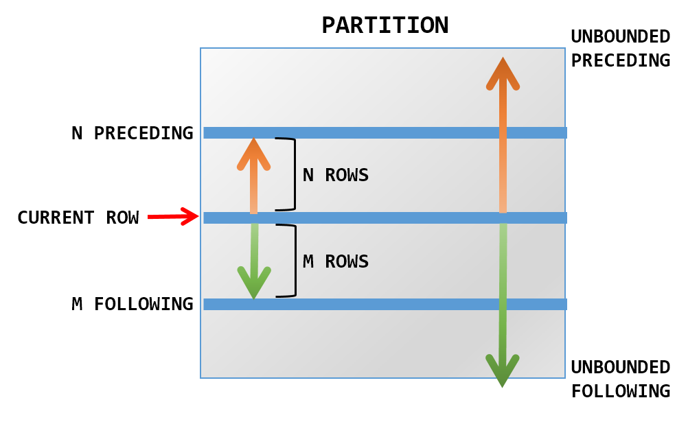
Common Frame Boundaries
| Boundary | Meaning |
|---|---|
UNBOUNDED PRECEDING |
From the first row in the partition |
CURRENT ROW |
The current row |
UNBOUNDED FOLLOWING |
Until the last row in the partition |
n PRECEDING |
n rows before |
n FOLLOWING |
n rows after |
Example 1: Running Total (Explicit Frame)
Example 1: Output
| sale_id | customer_id | sale_date | amount | running_total |
|---|---|---|---|---|
| 1 | A | 2024-01-01 | 100 | 100 |
| 2 | A | 2024-01-02 | 120 | 220 |
| 3 | A | 2024-01-03 | 90 | 310 |
| 4 | A | 2024-01-04 | 130 | 440 |
| 5 | B | 2024-01-01 | 180 | 180 |
| 6 | B | 2024-01-02 | 200 | 380 |
| 7 | B | 2024-01-03 | 220 | 600 |
| 8 | B | 2024-01-04 | 200 | 800 |
| 9 | C | 2024-01-01 | 150 | 150 |
| 10 | C | 2024-01-02 | 150 | 300 |
| 11 | C | 2024-01-03 | 170 | 470 |
| 12 | D | 2024-01-01 | 90 | 90 |
| 13 | D | 2024-01-02 | 110 | 200 |
| 14 | E | 2024-01-01 | 140 | 140 |
| 15 | E | 2024-01-02 | 160 | 300 |
| 16 | E | 2024-01-03 | 155 | 455 |
Example 2: Full-Partition Aggregate (Stable Value)
Example 2: Output
| sale_id | customer_id | amount | full_partition_avg |
|---|---|---|---|
| 1 | A | 100 | 110.000 |
| 2 | A | 120 | 110.000 |
| 3 | A | 90 | 110.000 |
| 4 | A | 130 | 110.000 |
| 5 | B | 180 | 200.000 |
| 6 | B | 200 | 200.000 |
| 7 | B | 220 | 200.000 |
| 8 | B | 200 | 200.000 |
| 9 | C | 150 | 156.667 |
| 10 | C | 150 | 156.667 |
| 11 | C | 170 | 156.667 |
| 12 | D | 90 | 100.000 |
| 13 | D | 110 | 100.000 |
| 14 | E | 140 | 151.667 |
| 15 | E | 160 | 151.667 |
| 16 | E | 155 | 151.667 |
Example 3: Moving Window (Last 2 Transactions)
Note
Here we can us any aggregate function: SUM(), MAX()
Example 3: Output
| sale_id | customer_id | sale_date | amount | moving_avg_2 |
|---|---|---|---|---|
| 1 | A | 2024-01-01 | 100 | 100.000 |
| 2 | A | 2024-01-02 | 120 | 110.000 |
| 3 | A | 2024-01-03 | 90 | 105.000 |
| 4 | A | 2024-01-04 | 130 | 110.000 |
| 5 | B | 2024-01-01 | 180 | 180.000 |
| 6 | B | 2024-01-02 | 200 | 190.000 |
| 7 | B | 2024-01-03 | 220 | 210.000 |
| 8 | B | 2024-01-04 | 200 | 210.000 |
| 9 | C | 2024-01-01 | 150 | 150.000 |
| 10 | C | 2024-01-02 | 150 | 150.000 |
| 11 | C | 2024-01-03 | 170 | 160.000 |
| 12 | D | 2024-01-01 | 90 | 90.000 |
| 13 | D | 2024-01-02 | 110 | 100.000 |
| 14 | E | 2024-01-01 | 140 | 140.000 |
| 15 | E | 2024-01-02 | 160 | 150.000 |
| 16 | E | 2024-01-03 | 155 | 157.500 |
Example 4: Forward-Looking Average
Example 4: Output
| sale_id | customer_id | sale_date | amount | forward_avg_2 |
|---|---|---|---|---|
| 1 | A | 2024-01-01 | 100 | 110.0000000000000000 |
| 2 | A | 2024-01-02 | 120 | 105.0000000000000000 |
| 3 | A | 2024-01-03 | 90 | 110.0000000000000000 |
| 4 | A | 2024-01-04 | 130 | 130.0000000000000000 |
| 5 | B | 2024-01-01 | 180 | 190.0000000000000000 |
| 6 | B | 2024-01-02 | 200 | 210.0000000000000000 |
| 7 | B | 2024-01-03 | 220 | 210.0000000000000000 |
| 8 | B | 2024-01-04 | 200 | 200.0000000000000000 |
| 9 | C | 2024-01-01 | 150 | 150.0000000000000000 |
| 10 | C | 2024-01-02 | 150 | 160.0000000000000000 |
| 11 | C | 2024-01-03 | 170 | 170.0000000000000000 |
| 12 | D | 2024-01-01 | 90 | 100.0000000000000000 |
| 13 | D | 2024-01-02 | 110 | 110.0000000000000000 |
| 14 | E | 2024-01-01 | 140 | 150.0000000000000000 |
| 15 | E | 2024-01-02 | 160 | 157.5000000000000000 |
| 16 | E | 2024-01-03 | 155 | 155.0000000000000000 |
Example 5: Centered Moving Average (Previous + Current + Next)
Example 5: Output
| sale_id | customer_id | sale_date | amount | centered_avg_3 |
|---|---|---|---|---|
| 1 | A | 2024-01-01 | 100 | 110.00 |
| 2 | A | 2024-01-02 | 120 | 103.33 |
| 3 | A | 2024-01-03 | 90 | 113.33 |
| 4 | A | 2024-01-04 | 130 | 110.00 |
| 5 | B | 2024-01-01 | 180 | 190.00 |
| 6 | B | 2024-01-02 | 200 | 200.00 |
| 7 | B | 2024-01-03 | 220 | 206.67 |
| 8 | B | 2024-01-04 | 200 | 210.00 |
| 9 | C | 2024-01-01 | 150 | 150.00 |
| 10 | C | 2024-01-02 | 150 | 156.67 |
| 11 | C | 2024-01-03 | 170 | 160.00 |
| 12 | D | 2024-01-01 | 90 | 100.00 |
| 13 | D | 2024-01-02 | 110 | 100.00 |
| 14 | E | 2024-01-01 | 140 | 150.00 |
| 15 | E | 2024-01-02 | 160 | 151.67 |
| 16 | E | 2024-01-03 | 155 | 157.50 |