Continuous Distributions
Probabilistic Distributions
Karen Hovhannisyan
2026-07-04
Well Known distributions
Topics
- Probabilistic Distributions
- Continuous Distributions
- Normal Distribution
- Uniform Distribution
- Exponential Distribution
What Is a Probabilistic Distribution?
In Data Analytics, we rarely know outcomes with certainty.
Instead of saying: “Tomorrow’s sales will be exactly 120 units”
We say: “Sales will most likely be around 120, but could reasonably vary”
What a Distribution Describes
A probabilistic distribution answers:
- What values can a variable take?
- How likely is each value (or range of values)?
- How is uncertainty spread across those values?
From Raw Data to Distribution
When we observe data repeatedly: - Customer purchases - Session durations - Delivery times
Patterns emerge.
A distribution summarizes these patterns as a model, not a table.
Random Variables
A random variable is a numerical description of uncertainty.
Examples:
- Number of purchases today
- Time until customer churns
- Email opened or not
Discrete vs Continuous
- Discrete: counted outcomes
- Purchases
- Complaints
- Click / no click
- Continuous: measured outcomes
- Revenue
- Time
- Weight
- Distance
Continuous Distributions
Most business variables are measured, not counted. Examples:
- Revenue
- Cost
- Time
- Duration
Continuous: Core Rule
Remember
For a continuous random variable \(X\): \[ P(X = x) = 0 \] Only intervals have probability: \[ P(a \le X \le b) \]
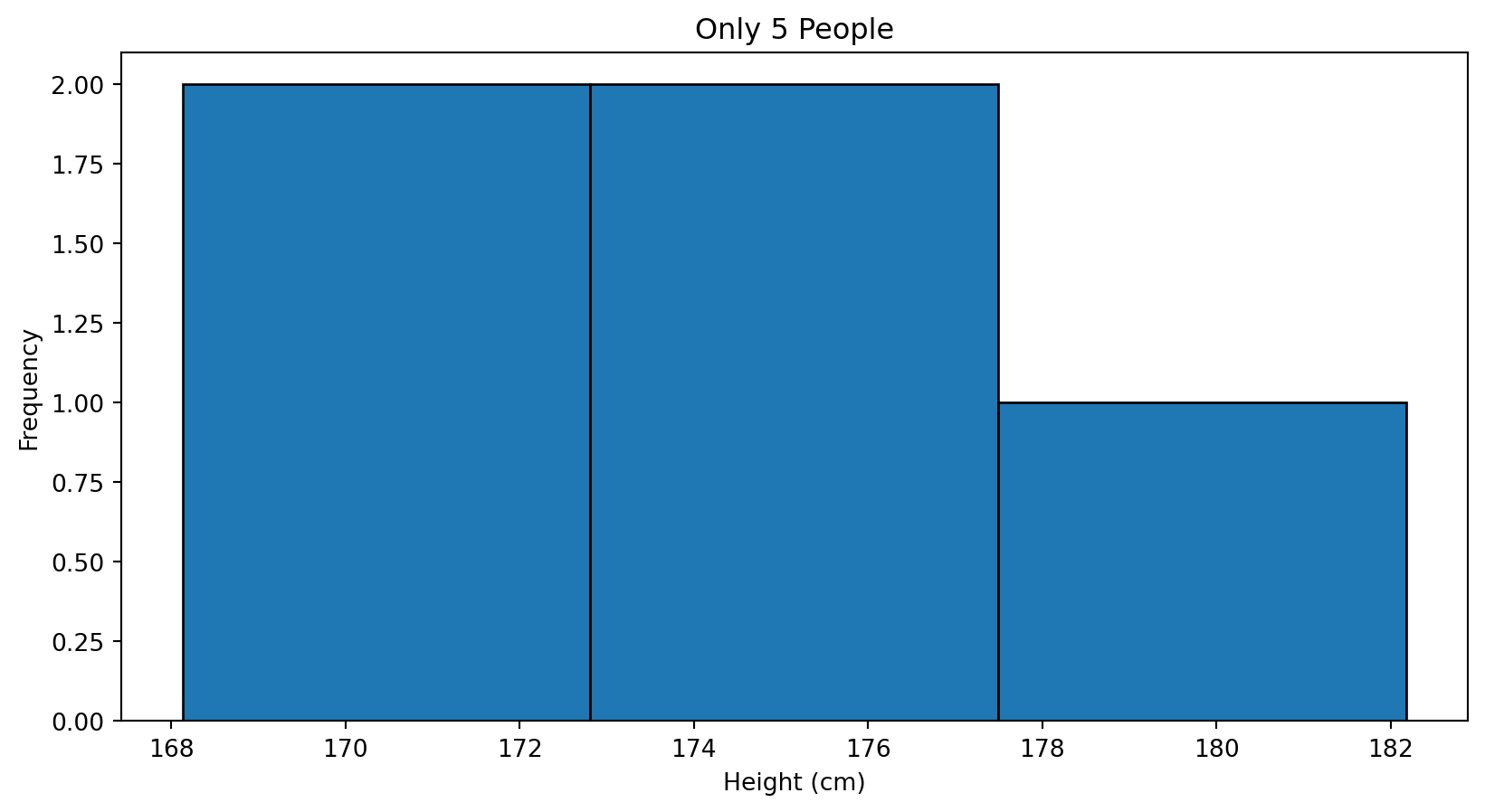
Example: Human Heights
Assume population height:
- Mean ≈ 170 cm
- Standard deviation ≈ 8 cm
We observe people one by one and build a distribution.
Small Sample → Noisy Picture
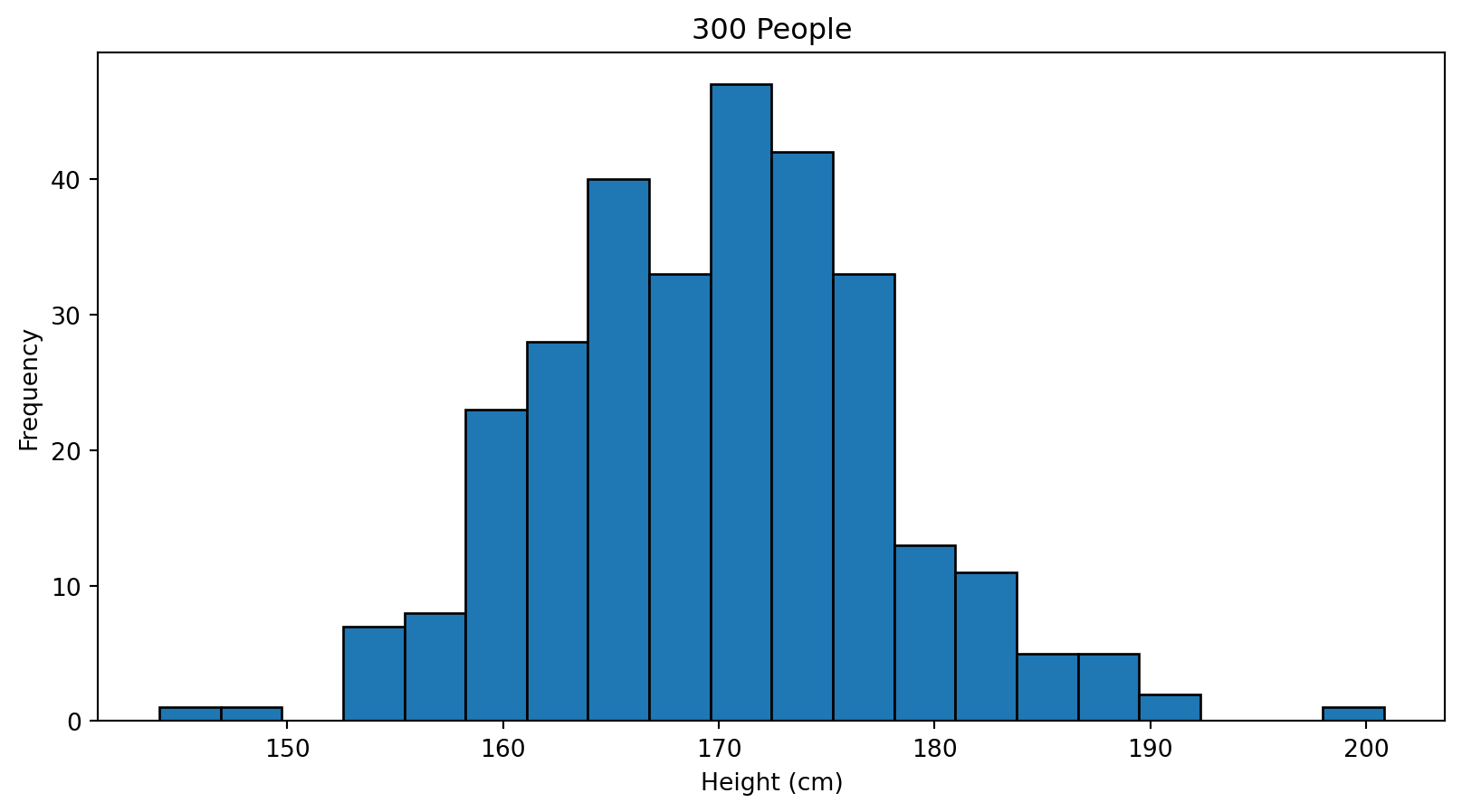
Larger Sample → Structure Emerges
Probability Density Function (PDF)
- PDF describes density, not probability
- Total area under the curve equals 1
- \[ \int_{-\infty}^{\infty} f(x)\,dx = 1 \]
Expected Value and Variance
Expected Value (Mean):
\[ E[X] = \int_{-\infty}^{\infty} x f(x)\,dx \]
Variance (Spread):
\[ Var(X) = \int_{-\infty}^{\infty} (x-\mu)^2 f(x)\,dx \]
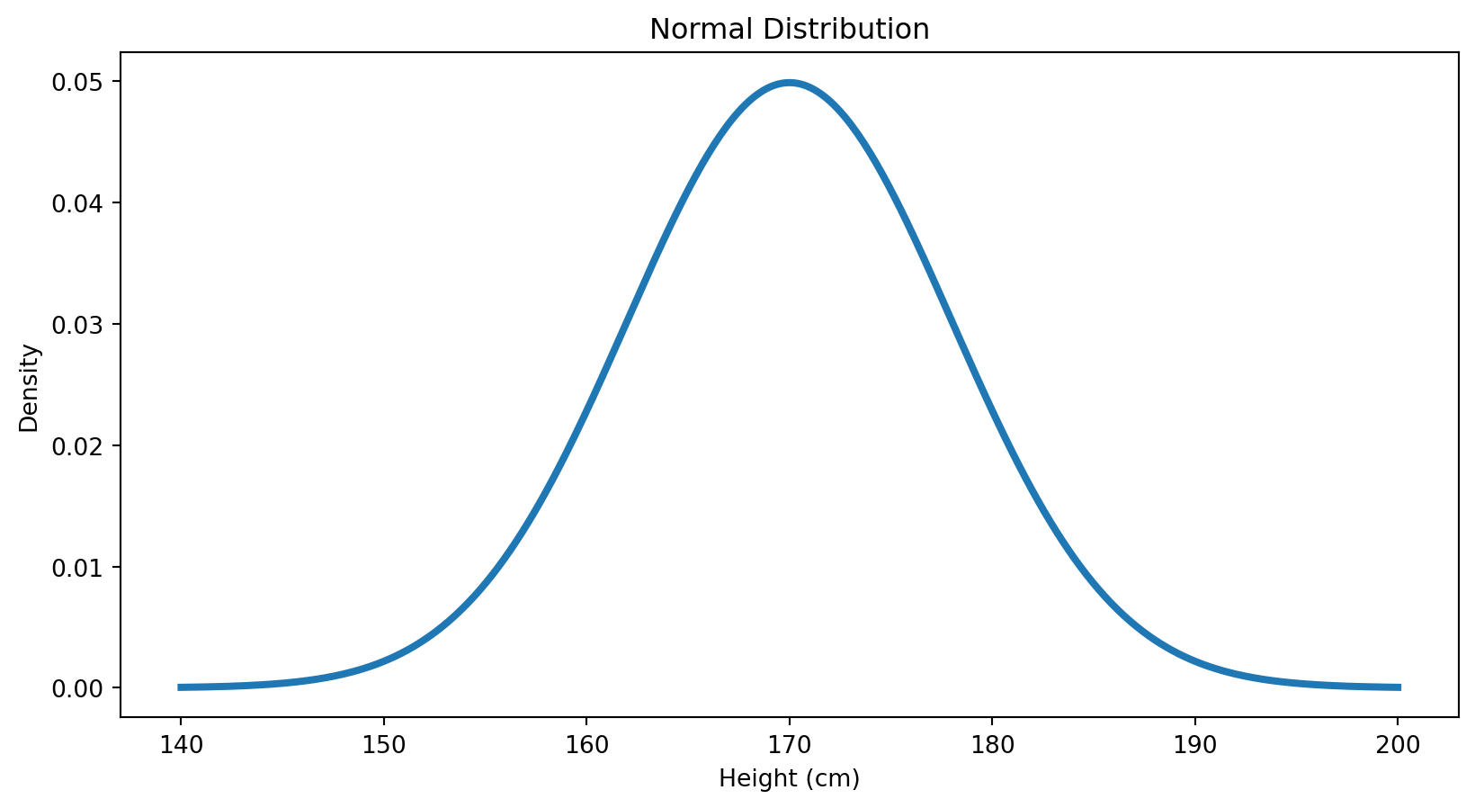
Normal Distribution
Definition
A Normal Distribution is:
- Symmetric
- Bell-shaped
- Fully defined by \(\mu\) and \(\sigma^2\)
\[ X \sim \mathcal{N}(\mu, \sigma^2) \]
Normal PDF
\[ f(x) = \frac{1}{\sigma\sqrt{2\pi}} \exp\!\left(-\frac{(x-\mu)^2}{2\sigma^2}\right) \]
Normal Distribution: Visualization
Standard Normal Distribution
Special case where:
\[ \mu = 0,\quad \sigma = 1 \]
\[ Z = \frac{X-\mu}{\sigma} \]
Normal vs Gaussian
Note
Normal and Gaussian distributions are the same thing.
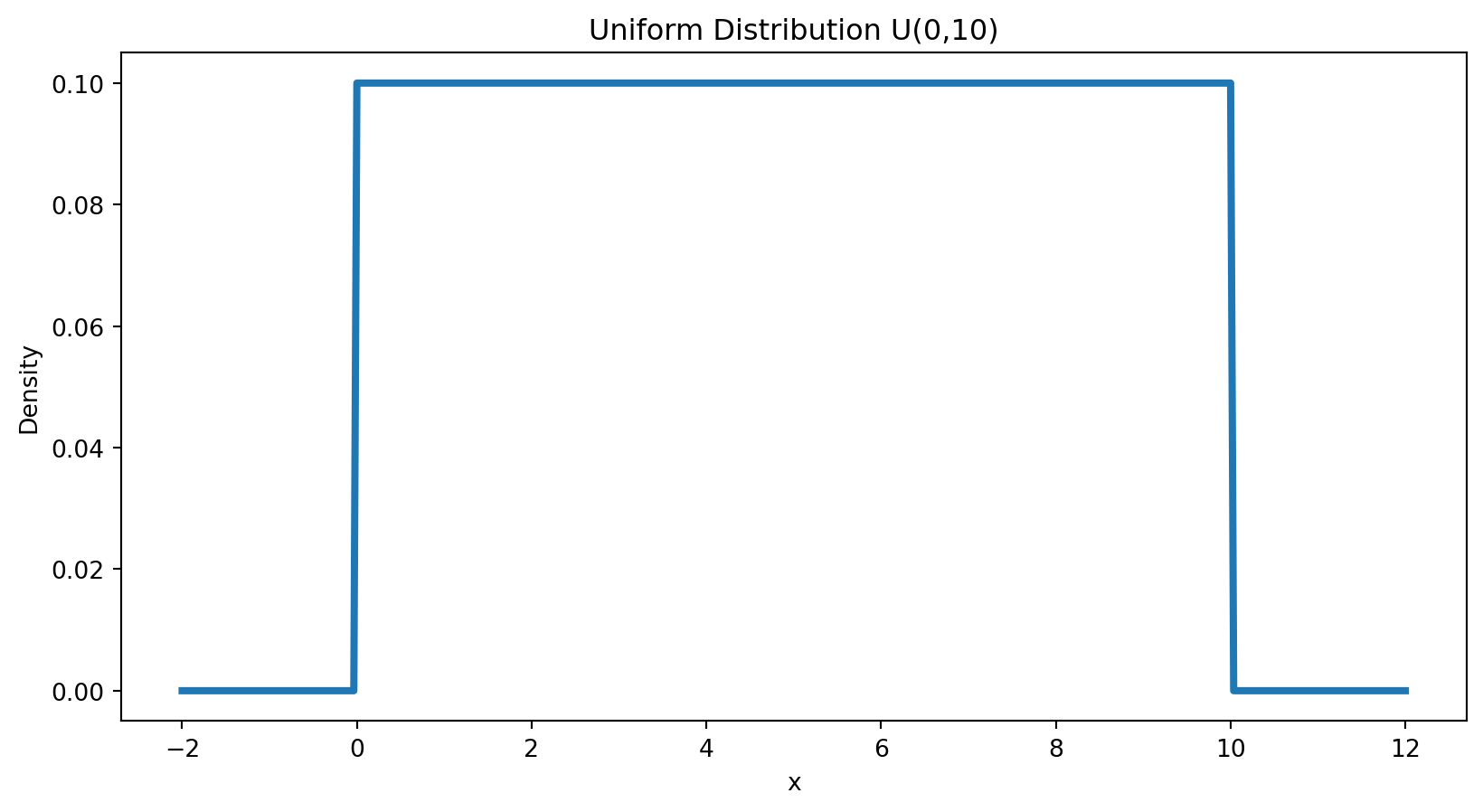
Uniform Distribution
Definition
\[ X \sim \text{Uniform}(a,b) \]
\[ f(x) = \frac{1}{b-a}, \quad a \le x \le b \]
Uniform Mean and Variance
\[ E[X] = \frac{a+b}{2} \]
\[ Var(X) = \frac{(b-a)^2}{12} \]
Uniform Visualization
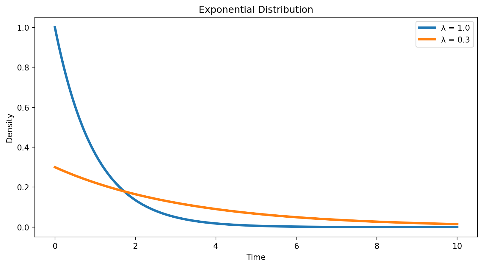
Exponential Distribution
Definition
Exponential distribution models waiting time until an event. \[ X \sim \text{Exp}(\lambda) \]
\[ f(x) = \lambda e^{-\lambda x}, \quad x \ge 0 \]
Exponential Mean and Variance
\[ E[X] = \frac{1}{\lambda} \]
\[ Var(X) = \frac{1}{\lambda^2} \]
Exponential Visualization
Summary
Spreadsheet Summary
Normal: =NORM.INV(RAND(),μ,σ), =NORM.DIST(x,μ,σ,TRUE)
Uniform: =RAND()*(b-a)+a
Exponential: =-LN(1-RAND())/λ
- Distributions model uncertainty
- Continuous variables require PDFs
- Normal, Uniform, Exponential model different behaviors
- Correct distribution choice drives correct decisions