Session 14: Clustering

Clustering

k-means

Segmentation

PCA

Learning objectives

Segmentation
Clustering
- K-means
- Hierarchical
- DBSCAN
Distance Metrics
- Euclidean
- Manhattan
- Pearson Correlation
Evaluation Metrics
- Elbow Method
- Silhouette analysis
Case Study

Customer Segmentation

Customer segmentation can be defined as the practice of dividing a customer base into groups of individuals that are similar in specific ways relevant to Marketing

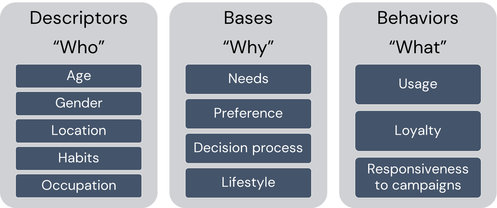
Why Segment Customers?

In one word: for differentiation!

Marketing and Service:
- Make more focused/targeted marketing
- Identify the most profitable and at-risk customers
- Build relationships
- Create user personas
Pruduct and Brand:
- Brand to appeal to particular segments
- Customize products and services
- Predict future purchasing patterns
Pricing:
- Pricing products by groups
- Determine Willingness to pay for optimal value

Important

There are number of ways for the customer segmentation, here we are going to do one using Clustering algorithms.

import pandas as pd
import numpy as np
import seaborn as sns
pd.set_option('display.max_columns', None)

Clustering

Customer segmentation can be achieved by using ML unsupervised learning algorithms

Unsupervised learning: No target variable, the goal is to discover patterns in data.

We are not going to discuss detailed technical aspects of the algorithms in the scope of the course, however the intuition and some evaluation metrics will be covered.

Apart from Customer Segmentation, the clustering algorithms are also used in:

Dimensionality Reduction
Feature Generation
Recommendation
Splitting Supervised ML algorithms

Clustering Algorithms are based on geometrical distances

Similarity and Distance

High level idea of clustering is to identify closest points. “The closeness” can be measured by number of distance metrics.

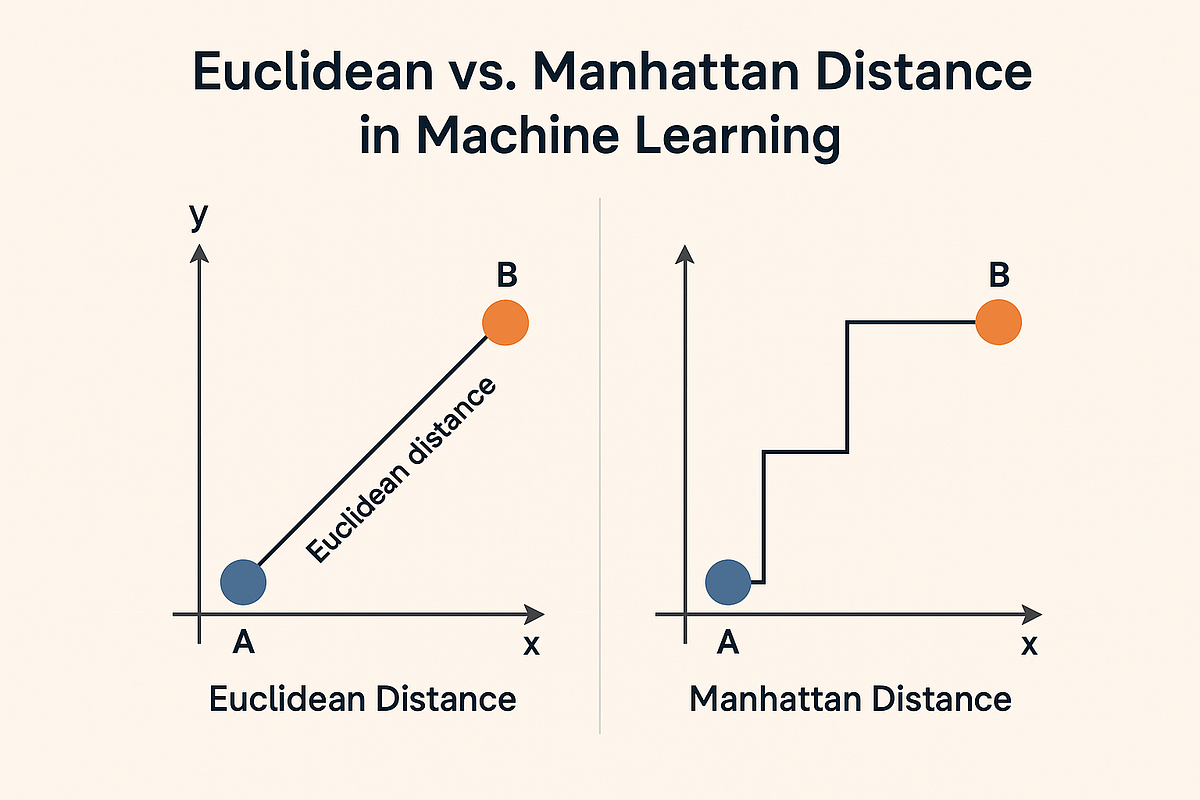
Those Distances could be in different types. The mose popular ones are:

Euclidean Distance
Manhattan Distance
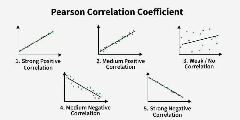
Pearson Correlation Distance

Euclidean distance

\[d_{euc}(x,y)=\sqrt{\sum_{i-1}^n(x_i-y_i)^2}\]

Manhattan distance

\[d_{man}(x,y)=\sum_{i-1}^n|x_i-y_i|\]

Pearson correlation distance:

\[d_{p.corr}(x,y)=1-\frac{\sum_{i-1}^n(x_i-\bar x)(y_i-\bar y)}{\sqrt{\sum_{i-1}^n(x_i-\bar x)^2 \sum_{i-1}^n(y_i-\bar y)^2 }}\]

Performance of Clustering Algorithms

There are 2 main groups of evaluation metrics:

External Measures: comparing with the ground truth labels
- Accuracy: \(acc(y,\hat y)=\frac{1}{n}\sum_{i=1}^{n-1}(\hat y_i=y_i)\)
- Homogeneity: A homogeneous clustering is one where each cluster has samples belonging the same class labels \(h=\frac{H(C/k)}{H(C)}\)
- Completeness: A complete clustering is one where all samples belonging to the same class as grouped into the same cluster \(c=\frac{H(K/C)}{H(K)}\)
- V-Measure: the harmonic mean between homogeneity and completeness: \(2\frac{hc}{h+c}\)
Internal Measures: quality of separation based on geometrical properties:
- Elbow Method
- Silhouette Coefficient

Cohesion: measures the distance of a point from the rest of the points within the cluster

Separation: measures the distance of point from cluster to the all points from other clusters

Clustering Set-Up

Problem set-up:

Result: assignment to clusters
Predictors: numerical and categorical

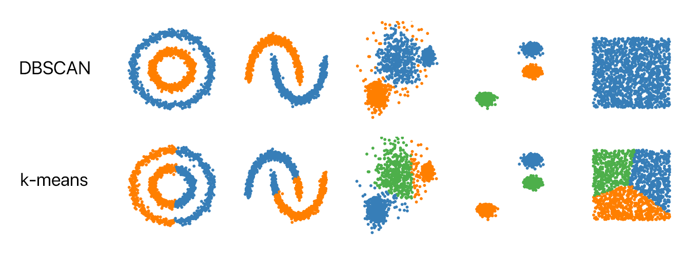
As mentioned there are lots of clustering algorithms, in the scope of the program we are going to work with K-Means Clustering.

K-Means Clustering

The most famous clustering algorithm.

Problem set-up:

Result: assignment to clusters (each observation to a single cluster)
Predictors: numerical
Pre-specified number of clusters!

Goal

Minimizing total within-cluster Euclidean distances:

\[W(C_k)=\sum_{x_i \in C_k}(x_i-\mu_k)^2\] \[minimize(\sum_{k=1}^k W(C_k))\]

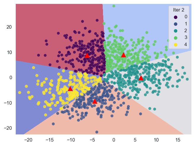
K-Means Steps

Choose the number \(K\) of clusters.
Select at random \(K\) points, the centroids, not necessarily from your data.
Assign each data point to the closest centroid.
Compute and place the new centroid of each cluster.
Reassign each data point to the new closest centroid. If any assignment took place, go to step 4; otherwise, finish.

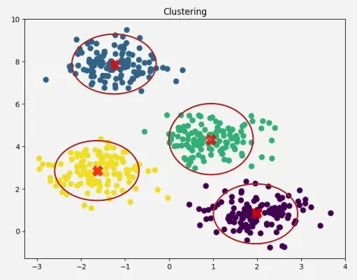
Checkout also the graphical explanation of the KMeans clustering below

With Fake Data

Fake Data

Let’s use make_blobs to create a 200 samples, of two classes with 3 centers

import matplotlib.pyplot as plt
from sklearn.datasets import make_blobs

X, Y = make_blobs(n_samples=200, n_features=2, centers=3, 
        cluster_std=1, shuffle=True, random_state=7)

plt.scatter(X[:, 0], X[:, 1], marker='o', s=70)
plt.show()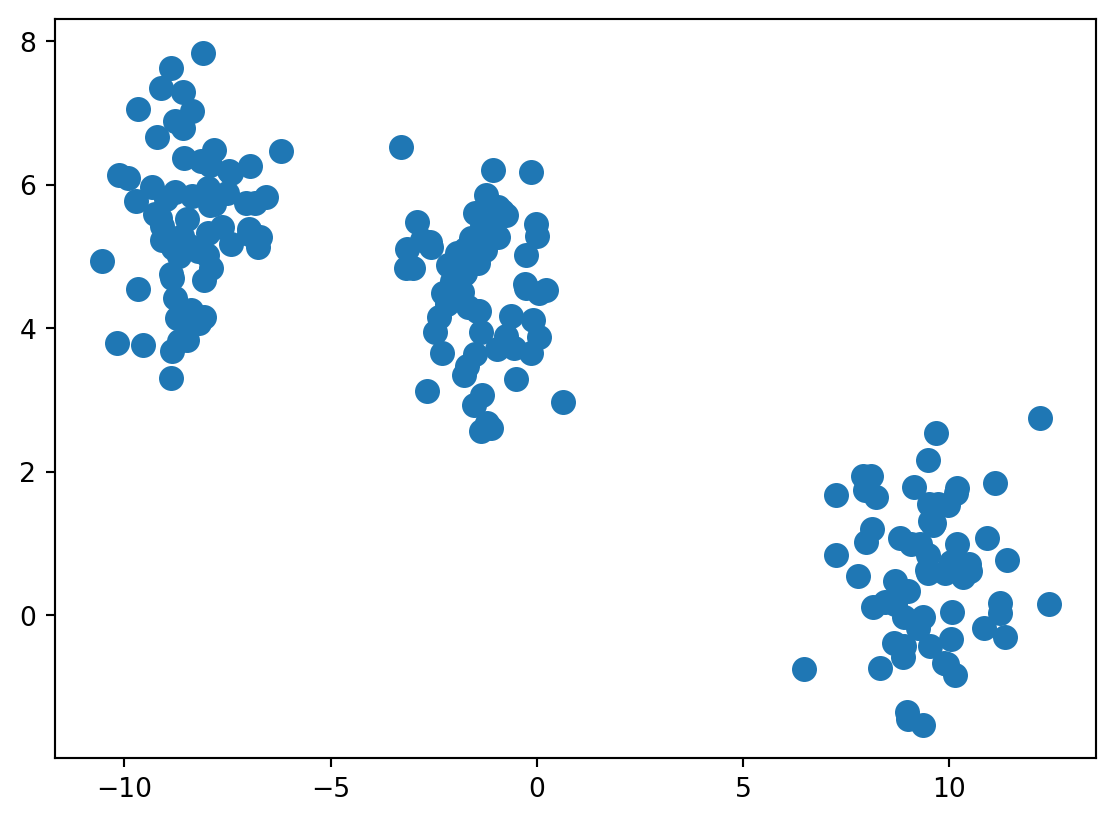

K-Means Fit

from sklearn.cluster import KMeans

km = KMeans(n_clusters=3, max_iter=500)
y_km = km.fit_predict(X)

# plot the 3 clusters
plt.scatter(X[y_km == 0, 0], X[y_km == 0, 1], c='lightgreen', label='cluster 1')
plt.scatter(X[y_km == 1, 0], X[y_km == 1, 1], c='orange',  label='cluster 2')
plt.scatter(X[y_km == 2, 0], X[y_km == 2, 1], c='lightblue',  label='cluster 3')

# plot the centroids
plt.scatter(km.cluster_centers_[:, 0], km.cluster_centers_[:, 1],
            s=250, marker='*',c='red', edgecolor='black',label='centroids')
plt.legend(scatterpoints=1)
plt.grid()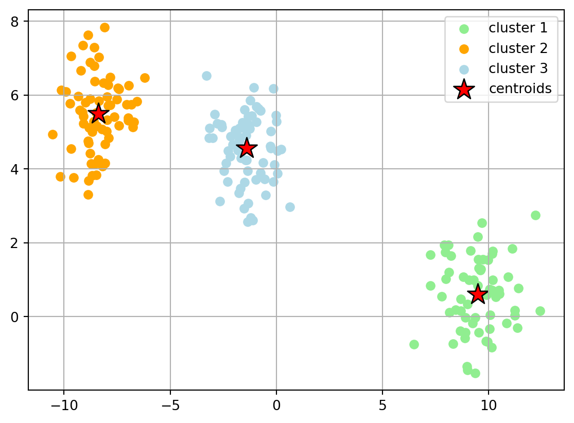

Optimal Number of Clusters

How to find out the optimal number of clusters, when there is no ground truth?

The only option is to use geometric properties of cluster:

Elbow method: Running the algorithm multiple times over a loop, with an increasing number of cluster choice and then plotting a *clustering score* as a function of the number of clusters. The point with Elbow like shape will show the optimal number of cluster.
Silhouette Analysis: the normalized average distance between points.

In the scope of segmentation, we are going to observe only those metrics.

Elbow Method

Sum_of_squared_distances = []
K = range(2,15)
for k in K:
    km = KMeans(n_clusters=k, init='random', n_init=10, max_iter=500,  tol=1e-04, random_state=0)
    km = km.fit(X)
    
    Sum_of_squared_distances.append(km.inertia_)

# Plot Results
plt.plot(K, Sum_of_squared_distances, marker='o')
plt.xlabel('k')
plt.ylabel('Sum_of_squared_distances')
plt.title('Elbow Method For Optimal k')
plt.show()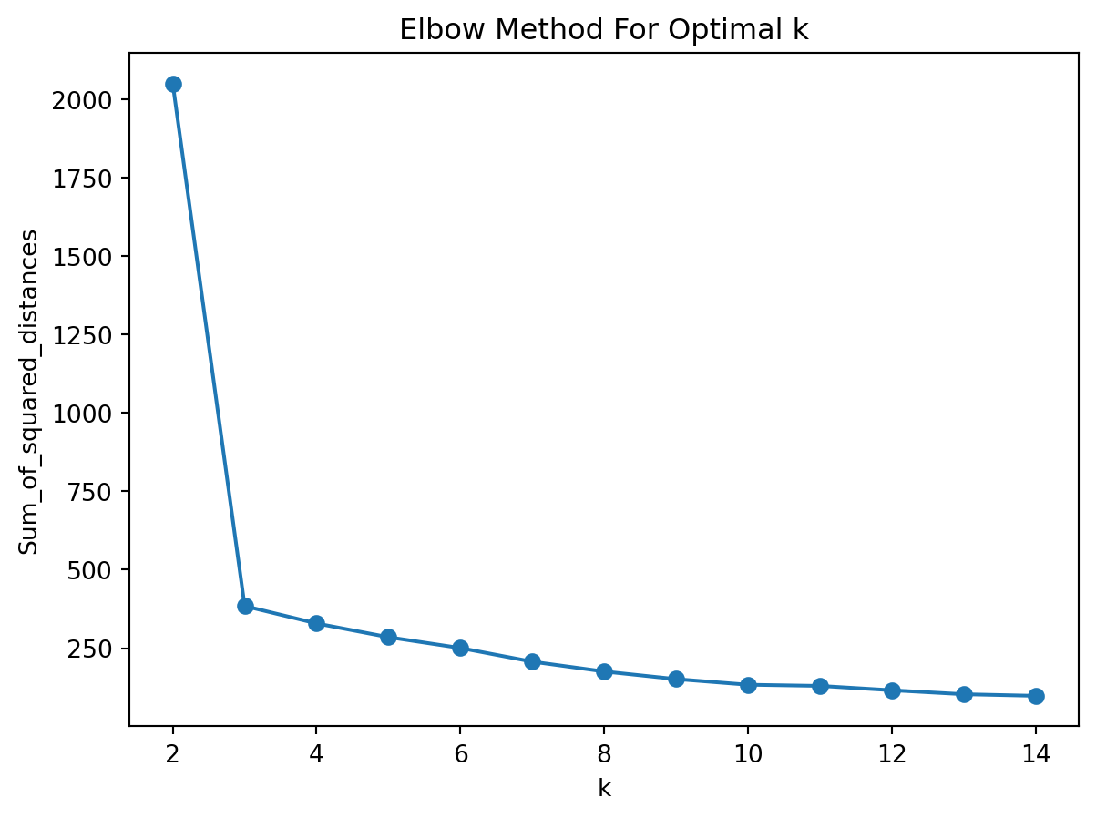

Silhouette Analysis

Clusters could be evaluated based on similarity or dissimilarity measure such as the distance between cluster point.

Silhouette Coefficient:

\[s=\frac{b-a}{max(a,b)}; [-1,1]\]

where:

\(a:\) the average distance from a point to other points within a cluster (intra-cluster)
\(b:\) the average distance from a point to the other closest cluster (extra-cluster)

when:

\(s=-1:\) misclassified
\(s=0:\) there is no difference between clusters
\(s=1:\) ideal split

Selecting the one which has the highest average silhouette score:

from sklearn.metrics import silhouette_score
for n_clusters in range(2,10):
    clusterer = KMeans(n_clusters=n_clusters, random_state=10)
    cluster_labels = clusterer.fit_predict(X)
    silhouette_avg = silhouette_score(X, cluster_labels)
    print("For n_clusters =", n_clusters,
          "The average silhouette_score is: {:4f}".format(silhouette_avg))

For n_clusters = 2 The average silhouette_score is: 0.748643
For n_clusters = 3 The average silhouette_score is: 0.785358
For n_clusters = 4 The average silhouette_score is: 0.641820
For n_clusters = 5 The average silhouette_score is: 0.461010
For n_clusters = 6 The average silhouette_score is: 0.477107
For n_clusters = 7 The average silhouette_score is: 0.325233
For n_clusters = 8 The average silhouette_score is: 0.478205
For n_clusters = 9 The average silhouette_score is: 0.361148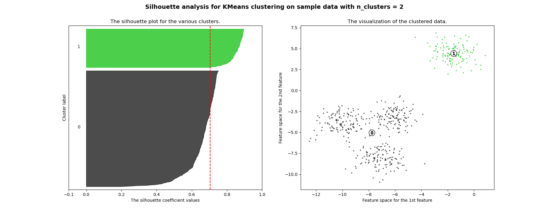

Tip

For more information you can visit here.

Other Clusering Methods

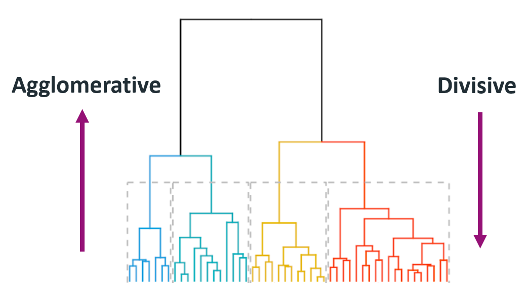
Hierarchical Clustering

Agglomerative (bottom-up): each observation starts as . Based on the distance of those clusters (in this case observations) it will merge into one cluster.
Divisive (Top-Bottom): starts at the top with The cluster will be partitioned at a point where it splits the big cluster into two big ones. This will get to a point where the observations cannot be split any more since each observation becomes its own cluster.

Steps

Make each data point a single point cluster (forms \(N\) cluster)
Take the 2 closes data point and make them 1 cluster (forms \(N-1\))
Take the 2 closest clusters and make them 1 cluster (\(N-2\) clusters)
Repeat step 3 until there is only 1 cluster
Finish

Intuition

DBSCAN

DBSCAN: Density Based Spatial Clustering of Applications with Noise.

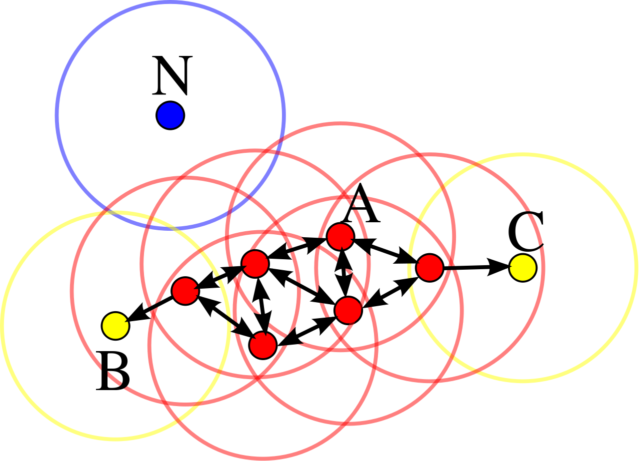
How it works?

Components:

\(\pmb{\epsilon:}\) indicates the radius of circular points
considering minimum points within the \({\epsilon}\)
In case of availability at least Min points, that point will be considered as Core Point
In case of availability at least one core point within the radios of epsilon
none of the above conditions are met

The algorithm works in a following way:

Select a random starting point: p
Finding Epsilon neighborhood of point p
- if it turns out core point, then cluster is formed
- if it is a border point, search other points, until all points in data are processed

Case Study

Clusering Travel Agency Booking Data

Our Goal is to find Customer Segments in order to help Marketing Team to target them more effectively!

Downloading The Data

df = pd.read_csv('https://raw.githubusercontent.com/hovhannisyan91/data_analytics_with_python/refs/heads/main/data/clustering/travel.csv',
parse_dates = ['date_time','srch_ci','srch_co'])
df.head()

	date_time	site_name	posa_continent	user_location_country	user_location_region	user_location_city	orig_destination_distance	user_id	is_package	channel	srch_ci	srch_co	srch_adults_cnt	srch_children_cnt	srch_rm_cnt	srch_destination_id	srch_destination_type_id	is_booking	cnt	hotel_continent	hotel_country	hotel_market	hotel_cluster
0	2014-11-03 16:02:00	24	2	77	871	36643	456.1151	792280	1	1	2014-12-15	2014-12-19	2	0	1	8286	1	0	1	0	63	1258	68
1	2013-03-13 19:25:00	11	3	205	135	38749	232.4737	961995	0	9	2013-03-13	2013-03-14	2	0	1	1842	3	0	1	2	198	786	37
2	2014-10-13 13:20:00	2	3	66	314	48562	4468.2720	495669	1	9	2015-04-03	2015-04-10	2	0	1	8746	1	0	1	6	105	29	22
3	2013-11-05 10:40:00	11	3	205	411	52752	171.6021	106611	0	0	2013-11-07	2013-11-08	2	0	1	6210	3	1	1	2	198	1234	42
4	2014-06-10 13:34:00	2	3	66	174	50644	NaN	596177	0	9	2014-08-03	2014-08-08	2	1	1	12812	5	0	1	2	50	368	83

Save

Do not forget to save the dataframe as csv

df.to_csv('../data/travel.csv')

Feature Descritpion

Column Name	Description	Data Type
date_time	Timestamp	string
site_name	ID of the Expedia point of sale	int
posa_continent	ID of continent associated with `site_name`	int
user_location_country	ID of the country the customer is located in	int
user_location_region	ID of the region the customer is located in	int
user_location_city	ID of the city the customer is located in	int
orig_destination_distance	Physical distance between a hotel and a customer at the time of search	double
user_id	ID of user	int
is_mobile	1 when a user connected from a mobile device, 0 otherwise	tinyint
is_package	1 if the click/booking was generated as part of a package, 0 otherwise	int
channel	ID of a marketing channel	int
srch_ci	Check-in date	string
srch_co	Check-out date	string
srch_adults_cnt	Number of adults specified in the hotel room	int
srch_children_cnt	Number of children specified in the hotel room	int
srch_rm_cnt	Number of hotel rooms specified in the search	int
srch_destination_id	ID of the destination where the hotel search was performed	int
srch_destination_type_id	Type of destination	int
hotel_continent	Hotel continent	int
hotel_country	Hotel country	int
hotel_market	Hotel market	int
cnt	Number of similar events in the context of the same user session	tinyint
hotel_cluster	ID of a hotel cluster	bigint
is_booking	1 if a booking, 0 if a click. This is what we are predicting	int

Dataframe Size

# Get some base information on our dataset
print ("Rows:   " , df.shape[0])
print ("Columns: " , df.shape[1])

Rows:    100000
Columns:  24

Information About df

df.info()

<class 'pandas.DataFrame'>
RangeIndex: 100000 entries, 0 to 99999
Data columns (total 24 columns):
 #   Column                     Non-Null Count   Dtype         
---  ------                     --------------   -----         
 0   date_time                  100000 non-null  datetime64[us]
 1   site_name                  100000 non-null  int64         
 2   posa_continent             100000 non-null  int64         
 3   user_location_country      100000 non-null  int64         
 4   user_location_region       100000 non-null  int64         
 5   user_location_city         100000 non-null  int64         
 6   orig_destination_distance  63915 non-null   float64       
 7   user_id                    100000 non-null  int64         
 8   is_mobile                  100000 non-null  int64         
 9   is_package                 100000 non-null  int64         
 10  channel                    100000 non-null  int64         
 11  srch_ci                    99878 non-null   datetime64[us]
 12  srch_co                    99878 non-null   datetime64[us]
 13  srch_adults_cnt            100000 non-null  int64         
 14  srch_children_cnt          100000 non-null  int64         
 15  srch_rm_cnt                100000 non-null  int64         
 16  srch_destination_id        100000 non-null  int64         
 17  srch_destination_type_id   100000 non-null  int64         
 18  is_booking                 100000 non-null  int64         
 19  cnt                        100000 non-null  int64         
 20  hotel_continent            100000 non-null  int64         
 21  hotel_country              100000 non-null  int64         
 22  hotel_market               100000 non-null  int64         
 23  hotel_cluster              100000 non-null  int64         
dtypes: datetime64[us](3), float64(1), int64(20)
memory usage: 18.3 MB

Missing Values

As we can see orig_destination_distance column has large amount of missing values. Taking into account, that we cannot infer anything from other features, we will simply remove the feature from further analysis.

# Get statistics for our Numerical Columns
df.isnull().sum()

date_time                        0
site_name                        0
posa_continent                   0
user_location_country            0
user_location_region             0
user_location_city               0
orig_destination_distance    36085
user_id                          0
is_mobile                        0
is_package                       0
channel                          0
srch_ci                        122
srch_co                        122
srch_adults_cnt                  0
srch_children_cnt                0
srch_rm_cnt                      0
srch_destination_id              0
srch_destination_type_id         0
is_booking                       0
cnt                              0
hotel_continent                  0
hotel_country                    0
hotel_market                     0
hotel_cluster                    0
dtype: int64

Correlation Matrix

Let’s see whic features are correlated. First we should build corr object and then visualize using heatmap from seaborn.

What could you infer?

# Create our Corelation Matrix
corr = df.corr()
corr

	date_time	site_name	posa_continent	user_location_country	user_location_region	user_location_city	orig_destination_distance	user_id	is_mobile	is_package	channel	srch_ci	srch_co	srch_adults_cnt	srch_children_cnt	srch_rm_cnt	srch_destination_id	srch_destination_type_id	is_booking	cnt	hotel_continent	hotel_country	hotel_market	hotel_cluster
date_time	1.000000	-0.024018	-0.010503	-0.021281	-0.012536	-0.004335	-0.002967	-0.017718	0.023642	-0.001773	-0.059976	0.952221	0.951117	0.013011	-0.075139	-0.004368	0.011650	-0.040562	-0.032699	-0.089140	-0.008460	-0.005722	0.003028	-0.000059
site_name	-0.024018	1.000000	-0.637743	0.159283	0.130818	-0.013471	0.027609	0.030404	-0.005418	0.048820	-0.027780	-0.001569	-0.001054	-0.013405	-0.031962	0.016585	0.034895	-0.006934	-0.013460	0.022274	0.201760	0.263167	-0.068316	-0.026689
posa_continent	-0.010503	-0.637743	1.000000	0.179726	-0.034647	0.039227	0.049808	-0.015209	0.016331	-0.093459	0.089680	-0.026851	-0.027669	0.012350	0.034453	-0.033712	-0.015535	0.037172	0.013319	-0.018952	-0.333578	-0.156578	0.049214	0.018297
user_location_country	-0.021281	0.159283	0.179726	1.000000	0.058496	0.122686	0.047689	-0.021091	0.003728	-0.025284	0.109999	-0.020851	-0.020539	0.042526	0.037101	0.000858	0.013486	0.028888	0.001284	0.003539	-0.063744	0.097624	0.015569	-0.011876
user_location_region	-0.012536	0.130818	-0.034647	0.058496	1.000000	0.132457	0.136560	0.002225	0.016982	0.040482	-0.001600	0.009723	0.010378	0.005487	0.014009	0.000254	0.022567	0.001376	0.000253	-0.007570	0.043027	-0.050301	0.040367	0.004984
user_location_city	-0.004335	-0.013471	0.039227	0.122686	0.132457	1.000000	0.014178	-0.007989	-0.003741	0.013032	0.023497	-0.004184	-0.003894	0.006628	0.002638	-0.000694	0.000786	-0.004399	-0.002655	-0.002175	0.007759	-0.001987	0.008558	0.000102
orig_destination_distance	-0.002967	0.027609	0.049808	0.047689	0.136560	0.014178	1.000000	0.017015	-0.059464	0.041991	-0.000398	0.080935	0.083821	-0.024039	-0.059722	-0.012484	-0.036314	-0.042859	-0.033480	0.009483	0.416180	0.254321	-0.090112	0.003624
user_id	-0.017718	0.030404	-0.015209	-0.021091	0.002225	-0.007989	0.017015	1.000000	-0.011439	-0.018901	-0.003593	-0.014944	-0.014900	-0.007370	0.002983	-0.001625	0.002716	0.007133	0.001561	0.001355	0.002447	0.008707	-0.002463	0.003202
is_mobile	0.023642	-0.005418	0.016331	0.003728	0.016982	-0.003741	-0.059464	-0.011439	1.000000	0.046903	-0.030770	0.024625	0.024727	0.016661	0.018211	-0.022565	-0.007140	-0.016039	-0.028623	0.008084	-0.024144	-0.029574	0.007644	0.012145
is_package	-0.001773	0.048820	-0.093459	-0.025284	0.040482	0.013032	0.041991	-0.018901	0.046903	1.000000	-0.011269	0.057690	0.061811	-0.024097	-0.037673	-0.036653	-0.146647	-0.224422	-0.081307	0.126500	0.108993	-0.044426	-0.014636	0.031399
channel	-0.059976	-0.027780	0.089680	0.109999	-0.001600	0.023497	-0.000398	-0.003593	-0.030770	-0.011269	1.000000	-0.071740	-0.071888	-0.014931	0.004202	0.010191	-0.000392	0.021612	0.025697	-0.010248	-0.022241	-0.001217	0.006164	0.002596
srch_ci	0.952221	-0.001569	-0.026851	-0.020851	0.009723	-0.004184	0.080935	-0.014944	0.024625	0.057690	-0.071740	1.000000	0.999897	0.042944	-0.054173	0.002106	-0.002510	-0.055652	-0.057114	-0.077000	0.029544	0.002502	-0.003590	0.008987
srch_co	0.951117	-0.001054	-0.027669	-0.020539	0.010378	-0.003894	0.083821	-0.014900	0.024727	0.061811	-0.071888	0.999897	1.000000	0.043023	-0.053617	0.001894	-0.003656	-0.056945	-0.058378	-0.076339	0.030990	0.002533	-0.003720	0.009516
srch_adults_cnt	0.013011	-0.013405	0.012350	0.042526	0.005487	0.006628	-0.024039	-0.007370	0.016661	-0.024097	-0.014931	0.042944	0.043023	1.000000	0.107061	0.525970	0.005651	-0.012119	-0.046350	0.014024	-0.019355	-0.018169	0.010203	0.006482
srch_children_cnt	-0.075139	-0.031962	0.034453	0.037101	0.014009	0.002638	-0.059722	0.002983	0.018211	-0.037673	0.004202	-0.054173	-0.053617	0.107061	1.000000	0.091711	-0.008784	-0.007217	-0.023228	0.019242	-0.061707	-0.045921	0.005056	0.021477
srch_rm_cnt	-0.004368	0.016585	-0.033712	0.000858	0.000254	-0.000694	-0.012484	-0.001625	-0.022565	-0.036653	0.010191	0.002106	0.001894	0.525970	0.091711	1.000000	0.018139	0.013618	0.009454	-0.000487	0.019150	0.011055	0.000104	-0.012177
srch_destination_id	0.011650	0.034895	-0.015535	0.013486	0.022567	0.000786	-0.036314	0.002716	-0.007140	-0.146647	-0.000392	-0.002510	-0.003656	0.005651	-0.008784	0.018139	1.000000	0.435605	0.027674	-0.021947	0.030365	0.053862	0.081240	-0.010406
srch_destination_type_id	-0.040562	-0.006934	0.037172	0.028888	0.001376	-0.004399	-0.042859	0.007133	-0.016039	-0.224422	0.021612	-0.055652	-0.056945	-0.012119	-0.007217	0.013618	0.435605	1.000000	0.037398	-0.024544	-0.035655	-0.021522	0.035783	-0.033039
is_booking	-0.032699	-0.013460	0.013319	0.001284	0.000253	-0.002655	-0.033480	0.001561	-0.028623	-0.081307	0.025697	-0.057114	-0.058378	-0.046350	-0.023228	0.009454	0.027674	0.037398	1.000000	-0.108628	-0.025629	-0.004763	0.012633	-0.018192
cnt	-0.089140	0.022274	-0.018952	0.003539	-0.007570	-0.002175	0.009483	0.001355	0.008084	0.126500	-0.010248	-0.077000	-0.076339	0.014024	0.019242	-0.000487	-0.021947	-0.024544	-0.108628	1.000000	0.020670	0.001443	-0.008747	-0.000607
hotel_continent	-0.008460	0.201760	-0.333578	-0.063744	0.043027	0.007759	0.416180	0.002447	-0.024144	0.108993	-0.022241	0.029544	0.030990	-0.019355	-0.061707	0.019150	0.030365	-0.035655	-0.025629	0.020670	1.000000	0.295991	-0.096278	-0.015632
hotel_country	-0.005722	0.263167	-0.156578	0.097624	-0.050301	-0.001987	0.254321	0.008707	-0.029574	-0.044426	-0.001217	0.002502	0.002533	-0.018169	-0.045921	0.011055	0.053862	-0.021522	-0.004763	0.001443	0.295991	1.000000	0.017868	-0.025002
hotel_market	0.003028	-0.068316	0.049214	0.015569	0.040367	0.008558	-0.090112	-0.002463	0.007644	-0.014636	0.006164	-0.003590	-0.003720	0.010203	0.005056	0.000104	0.081240	0.035783	0.012633	-0.008747	-0.096278	0.017868	1.000000	0.037060
hotel_cluster	-0.000059	-0.026689	0.018297	-0.011876	0.004984	0.000102	0.003624	0.003202	0.012145	0.031399	0.002596	0.008987	0.009516	0.006482	0.021477	-0.012177	-0.010406	-0.033039	-0.018192	-0.000607	-0.015632	-0.025002	0.037060	1.000000

plt.figure(figsize = (10,10))

sns.heatmap(corr,xticklabels=corr.columns.values,
           yticklabels=corr.columns.values,vmax=.3, center=0, square=True, linewidths=.5, cbar_kws={"shrink": .82})
plt.title('Heatmap of Correlation Matrix')

Text(0.5, 1.0, 'Heatmap of Correlation Matrix')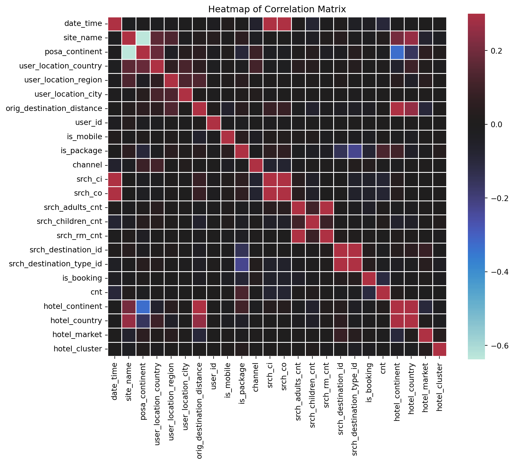

Distributions

What could you say about this?

df[['channel', 'is_booking', 'is_mobile', 'orig_destination_distance',
        'srch_rm_cnt', 'srch_adults_cnt', 'srch_children_cnt']].hist(figsize=(10,12))

array([[<Axes: title={'center': 'channel'}>,
        <Axes: title={'center': 'is_booking'}>,
        <Axes: title={'center': 'is_mobile'}>],
       [<Axes: title={'center': 'orig_destination_distance'}>,
        <Axes: title={'center': 'srch_rm_cnt'}>,
        <Axes: title={'center': 'srch_adults_cnt'}>],
       [<Axes: title={'center': 'srch_children_cnt'}>, <Axes: >,
        <Axes: >]], dtype=object)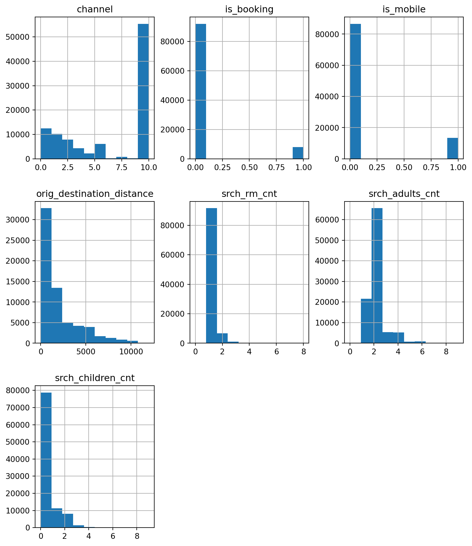

`is_booking`

# To view the bookings made per user
booking_count_per_user=df.groupby('user_id')['is_booking'].agg(num_of_bookings='count').reset_index()
booking_count_per_user.groupby('num_of_bookings')['user_id'].agg('count')

num_of_bookings
1    79189
2     8423
3     1065
4      161
5       24
6        1
Name: user_id, dtype: int64

Merge with the Original Data

df = df.merge(df.groupby('user_id')['is_booking'].agg(['count']).reset_index())
df.head()

	date_time	site_name	posa_continent	user_location_country	user_location_region	user_location_city	orig_destination_distance	user_id	is_package	channel	srch_ci	srch_co	srch_adults_cnt	srch_children_cnt	srch_rm_cnt	srch_destination_id	srch_destination_type_id	is_booking	cnt	hotel_continent	hotel_country	hotel_market	hotel_cluster	count
0	2014-11-03 16:02:00	24	2	77	871	36643	456.1151	792280	1	1	2014-12-15	2014-12-19	2	0	1	8286	1	0	1	0	63	1258	68	2
1	2013-03-13 19:25:00	11	3	205	135	38749	232.4737	961995	0	9	2013-03-13	2013-03-14	2	0	1	1842	3	0	1	2	198	786	37	1
2	2014-10-13 13:20:00	2	3	66	314	48562	4468.2720	495669	1	9	2015-04-03	2015-04-10	2	0	1	8746	1	0	1	6	105	29	22	1
3	2013-11-05 10:40:00	11	3	205	411	52752	171.6021	106611	0	0	2013-11-07	2013-11-08	2	0	1	6210	3	1	1	2	198	1234	42	2
4	2014-06-10 13:34:00	2	3	66	174	50644	NaN	596177	0	9	2014-08-03	2014-08-08	2	1	1	12812	5	0	1	2	50	368	83	1

Logical Check

Remember, Data Analysts cannot take data and immidetly start modeling. It is expected from the data professioanl to acquire domain knowledge.

Available Travelers

Taking into account that number of travelers should be greater then 0, we must remove 174 cases fro the data. Let’s drop such cases.

pd.crosstab(df['srch_adults_cnt'], df['srch_children_cnt'])

srch_children_cnt	0	1	2	3	4	5	6	7	8	9
srch_adults_cnt
0	174	2	3	2	0	0	0	0	0	0
1	18749	2137	523	117	11	1	9	1	2	0
2	50736	7093	6529	972	208	14	7	1	0	0
3	3645	1131	469	131	27	5	2	2	0	2
4	3933	690	494	77	83	9	4	0	0	0
5	535	131	41	20	6	4	2	0	0	0
6	669	73	53	28	18	13	7	0	0	0
7	99	20	5	8	6	3	0	0	0	0
8	183	12	13	2	6	1	3	2	2	1
9	24	5	4	2	1	1	2	0	0	0

Let’s view those cases

df[(df['srch_adults_cnt']==0) & (df['srch_children_cnt']==0)].head()

	date_time	site_name	posa_continent	user_location_country	user_location_region	user_location_city	orig_destination_distance	user_id	is_mobile	is_package	channel	srch_ci	srch_co	srch_rm_cnt	srch_destination_id	srch_destination_type_id	cnt	hotel_continent	hotel_country	hotel_market	hotel_cluster	count
115	2014-10-07 14:43:00	2	3	66	293	52284	NaN	909952	0	1	9	2015-01-10	2015-01-15	1	8250	1	1	2	50	628	1	1
496	2013-06-15 19:12:00	29	1	52	40	29080	NaN	150434	0	1	9	2013-09-16	2013-09-20	2	25408	6	2	6	15	1534	46	1
1261	2014-10-26 10:20:00	2	3	66	220	22648	5148.4830	588617	1	1	2	2015-08-24	2015-09-03	1	8746	1	1	6	105	29	78	1
1428	2014-11-16 10:21:00	2	3	66	174	53801	1638.7472	207522	1	1	0	2015-04-18	2015-04-25	1	8810	1	1	4	8	1532	52	1
1539	2014-12-28 19:16:00	2	3	66	363	31138	1526.8518	938404	0	1	0	NaT	NaT	1	8277	1	1	2	50	412	9	1

df[(df['srch_adults_cnt']==0) & (df['srch_children_cnt']==0)].shape

(174, 25)

Once we got confirmed that everything is correct and working, we can drop those rows with inplace = True

df.drop(df[df['srch_adults_cnt'] + df['srch_children_cnt']==0].index, inplace=True)

Dates

Converting string objects into datatime objects. And creating new date column from date_time. (We did this during the import )

The chronology: Booking \(\rightarrow\) Check-In \(\rightarrow\) Check-out

Check-out date need to be later than check-in date
Check-in date need to be later than booking date

Change the timestamp of ‘date_time’ (2014-11-03 16:02:28) to simply "2014-11-03"

df['date'] = pd.to_datetime(df['date_time'].apply(lambda x: x.date()))

df.head()

	date_time	site_name	posa_continent	user_location_country	user_location_region	user_location_city	orig_destination_distance	user_id	is_package	channel	srch_ci	srch_co	srch_adults_cnt	srch_children_cnt	srch_rm_cnt	srch_destination_id	srch_destination_type_id	is_booking	cnt	hotel_continent	hotel_country	hotel_market	hotel_cluster	count	date
0	2014-11-03 16:02:00	24	2	77	871	36643	456.1151	792280	1	1	2014-12-15	2014-12-19	2	0	1	8286	1	0	1	0	63	1258	68	2	2014-11-03
1	2013-03-13 19:25:00	11	3	205	135	38749	232.4737	961995	0	9	2013-03-13	2013-03-14	2	0	1	1842	3	0	1	2	198	786	37	1	2013-03-13
2	2014-10-13 13:20:00	2	3	66	314	48562	4468.2720	495669	1	9	2015-04-03	2015-04-10	2	0	1	8746	1	0	1	6	105	29	22	1	2014-10-13
3	2013-11-05 10:40:00	11	3	205	411	52752	171.6021	106611	0	0	2013-11-07	2013-11-08	2	0	1	6210	3	1	1	2	198	1234	42	2	2013-11-05
4	2014-06-10 13:34:00	2	3	66	174	50644	NaN	596177	0	9	2014-08-03	2014-08-08	2	1	1	12812	5	0	1	2	50	368	83	1	2014-06-10

Checking the logic between the check-ins and check-outs

df[df['srch_co'] < df['srch_ci']][['srch_co', 'srch_ci']].shape

(2, 2)

Checkin the logic between the book_date and check-in

df[df['srch_ci'] < df['date']][['srch_ci', 'date']].shape

(25, 2)

Feature Enrichment

In order to get to remove thos cases, first let’s create two important (at least from business perspective) features from existing date columns, by applying duration() function:

duration
days_in_advance

Creating duration() function

def duration(row,start, end):
    delta=(row[end]-row[start])/np.timedelta64(1,'D')
    if delta<=0:
        return np.nan
    else:
        return delta

Duration is finds the length of stay by substracting the checkout day from the checkin day

df['duration'] = df.apply(duration, args=('srch_ci','srch_co'),axis=1)

Shows how long in advance the booking was made. Done by substracting the checkin date from the booking date

df['days_in_advance'] = df.apply(duration,args=('date','srch_ci'), axis=1)

Statistical Analysis of Booking Channels

Let’s look at how each channel performs by seeing the booking rate for each channel type.

booking rate per channel

(df
    .groupby('channel')['is_booking']
    .agg(booking_rate= 'mean', num_of_bookings= 'count')
    .reset_index()
    .sort_values(by='channel'))

	channel	booking_rate	num_of_bookings
0	0	0.072184	12482
1	1	0.069568	10249
2	2	0.060583	7824
3	3	0.060482	4398
4	4	0.120438	2192
5	5	0.094533	6146
6	6	0.068323	161
7	7	0.043263	809
8	8	0.051852	270
9	9	0.085365	55280
10	10	0.200000	15

Clustering

Let’s choose some features using our business domain knowledge and explore these. After selecting features, let’s create two new dataframes with our new data called:

df_clustering
df_clustering_groups grouped by user_location_city

Note: you’re free to add and remove

Feature Selection

# Our selected features
features_to_explore = ['duration', 'days_in_advance', 'orig_destination_distance', 'is_mobile',
            'is_package', 'srch_adults_cnt', 'srch_children_cnt', 'srch_rm_cnt']


df_clustering = df[features_to_explore + ['user_location_city']]

df_clustering_groups = (df_clustering
                            .groupby('user_location_city')
                            .mean()
                            .reset_index()
                            .dropna(axis=0))

Standardize our Data

Let’s keep copy df_clustering_groups dataset, in order to keep the original one for post-analysis.

Clustering algorithms try to group similar observations together. To do this, they usually measure the distance between data points.

The problem is that different variables can have very different scales.

For example, imagine we are clustering customers using two columns:

Customer	Age	Annual Income
A	25	20,000
B	45	80,000
C	50	85,000

Important

Here, age ranges from around 20 to 60, while income ranges from thousands to tens of thousands.

Without standardization, the clustering algorithm may think that income is much more important than age simply because the numbers are larger.

Suppose we compare two customers:

Feature	Difference
Age difference	10 years
Income difference	30,000

The algorithm sees: \(30,000 \gg 10\)

So the income difference dominates the distance calculation.

But this does not necessarily mean income is more important. It only means income is measured on a larger scale.

What Standardization Does

Standardization transforms each numeric column so that it has:

mean equal to \(0\)
standard deviation equal to \(1\)

The common formula is:

\[ z = \frac{x - \mu}{\sigma} \]

Where:

\(x\) is the original value
\(\mu\) is the mean of the column
\(\sigma\) is the standard deviation of the column

After standardization, all numeric variables are put on a comparable scale.

Important

Thus, standardization helps clustering algorithms treat variables more fairly.

Without standardization:

variables with large values dominate the clustering
distance calculations become misleading
clusters may reflect scale, not real similarity
the results may be hard to interpret correctly

With standardization:

each variable contributes more equally
distance calculations become more meaningful
clusters are based on patterns, not just large numbers
the algorithm can better identify real groups in the data

from sklearn import preprocessing
df_clustering_std = df_clustering_groups.copy()

df_clustering_std[features_to_explore] = preprocessing.scale(df_clustering_std[features_to_explore])

df_clustering_std.head()

	user_location_city	duration	days_in_advance	orig_destination_distance	is_mobile	is_package	srch_adults_cnt	srch_children_cnt	srch_rm_cnt
0	0	-0.685258	0.447140	0.314747	-0.619979	-0.023150	-0.511139	-0.704997	-0.331661
2	3	0.564013	0.651185	1.020233	-0.347544	0.125553	-0.207376	0.201429	-0.331661
3	7	5.164984	-0.007237	2.600430	-0.619979	2.504801	-0.113910	-0.704997	-0.331661
5	14	1.752343	-0.500401	2.195332	-0.619979	-0.865800	-0.113910	0.739619	-0.331661
8	21	0.777303	-0.594601	0.221515	-0.619979	0.819500	-0.908368	1.221158	-0.331661

K-means Clustering

Let’s start K-means clustering and initially selectK=3!

Creating cluster column for the same dataset

km = KMeans(n_clusters=3, max_iter=300, random_state=123)
df_clustering_std['cluster'] = km.fit_predict(df_clustering_std[features_to_explore])

df_clustering_std.head()

	user_location_city	duration	days_in_advance	orig_destination_distance	is_mobile	is_package	srch_adults_cnt	srch_children_cnt	srch_rm_cnt	cluster
0	0	-0.685258	0.447140	0.314747	-0.619979	-0.023150	-0.511139	-0.704997	-0.331661	2
2	3	0.564013	0.651185	1.020233	-0.347544	0.125553	-0.207376	0.201429	-0.331661	1
3	7	5.164984	-0.007237	2.600430	-0.619979	2.504801	-0.113910	-0.704997	-0.331661	0
5	14	1.752343	-0.500401	2.195332	-0.619979	-0.865800	-0.113910	0.739619	-0.331661	1
8	21	0.777303	-0.594601	0.221515	-0.619979	0.819500	-0.908368	1.221158	-0.331661	0

Principal Component Analysis (PCA)

It is a technique used to reduce the number of variables in a dataset while keeping as much useful information as possible.

In simple terms, PCA tries to find the most important directions in the data.

These directions are called principal components.

PCA takes many related variables and creates a smaller number of new variables that still keep most of the important information.

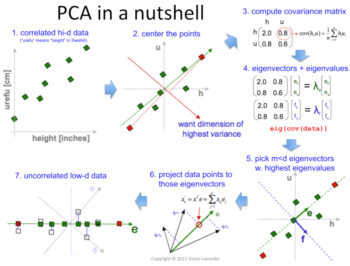
One common use of PCA is visualization.

If a dataset has 10 or 20 columns, we cannot easily plot it.

But PCA can reduce the data into 2 components and we are going to do exactly the same!

from sklearn import decomposition

pca = decomposition.PCA(n_components=2, whiten=True)

pca_results = pca.fit_transform(df_clustering_std[features_to_explore])

explained_variance = pca.explained_variance_ratio_
cumulative_variance = np.cumsum(explained_variance)


print(f"Comulative Variance:  {cumulative_variance}")
explained_variance

Comulative Variance:  [0.21982537 0.40991447]

array([0.21982537, 0.1900891 ])

40% of the variance is explaned by two columns!

df_clustering_std['x'] = pca_results[:,0]
df_clustering_std['y'] = pca_results[:,1]

df_clustering_std.head()

	user_location_city	duration	days_in_advance	orig_destination_distance	is_mobile	is_package	srch_adults_cnt	srch_children_cnt	srch_rm_cnt	cluster	x	y
0	0	-0.685258	0.447140	0.314747	-0.619979	-0.023150	-0.511139	-0.704997	-0.331661	2	0.095833	-0.521284
2	3	0.564013	0.651185	1.020233	-0.347544	0.125553	-0.207376	0.201429	-0.331661	1	0.929255	-0.156800
3	7	5.164984	-0.007237	2.600430	-0.619979	2.504801	-0.113910	-0.704997	-0.331661	0	3.937174	-0.238704
5	14	1.752343	-0.500401	2.195332	-0.619979	-0.865800	-0.113910	0.739619	-0.331661	1	1.051649	-0.087671
8	21	0.777303	-0.594601	0.221515	-0.619979	0.819500	-0.908368	1.221158	-0.331661	0	0.425947	-0.558020

Now we can visualize thos cluseters!

plt.scatter(df_clustering_std['x'], df_clustering_std['y'], c=df_clustering_std['cluster'])
plt.show()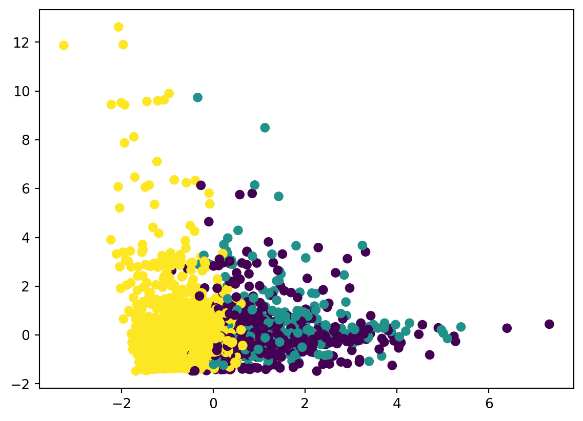

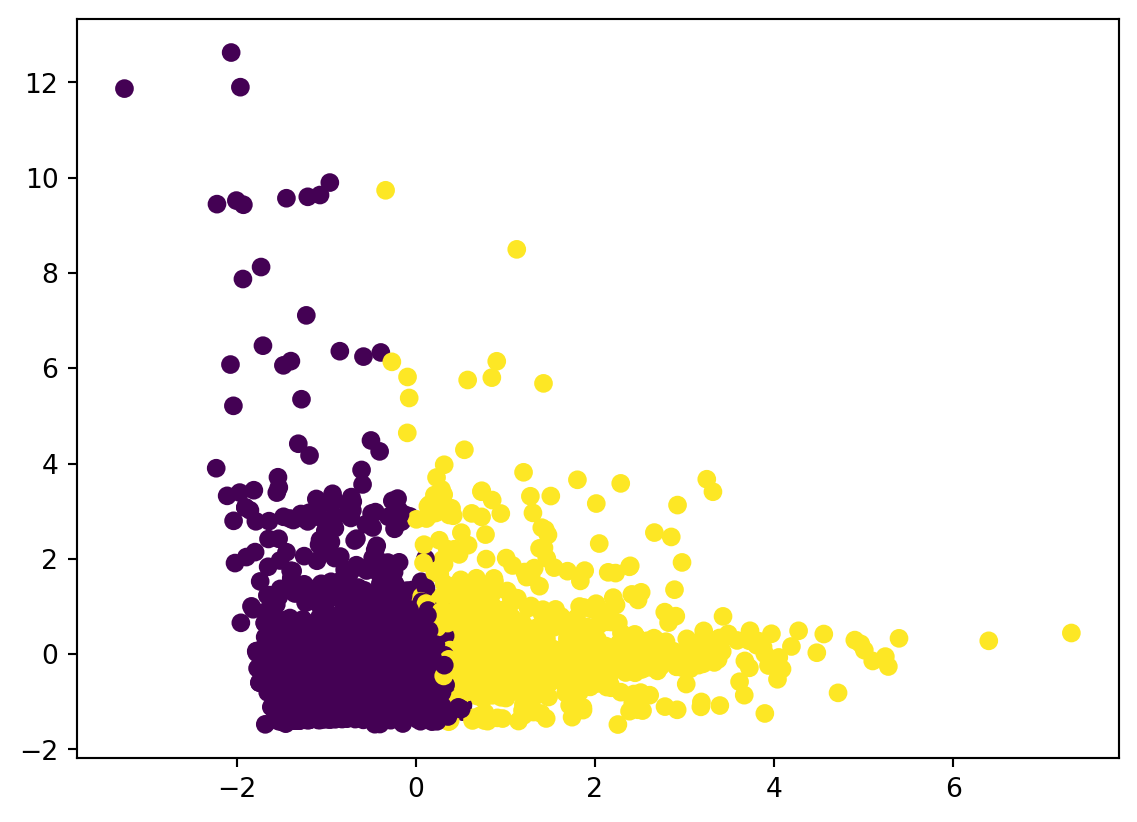
with `2` clusters

km = KMeans(n_clusters=2, max_iter=300, random_state=None)
df_clustering_std['cluster'] = km.fit_predict(df_clustering_std[features_to_explore])

pca = decomposition.PCA(n_components=2, whiten=True)
pca_results = pca.fit_transform(df_clustering_std[features_to_explore])

df_clustering_std['x'] = pca_results[:,0]
df_clustering_std['y'] = pca_results[:,1]

plt.scatter(df_clustering_std['x'], df_clustering_std['y'], c=df_clustering_std['cluster'])
plt.show()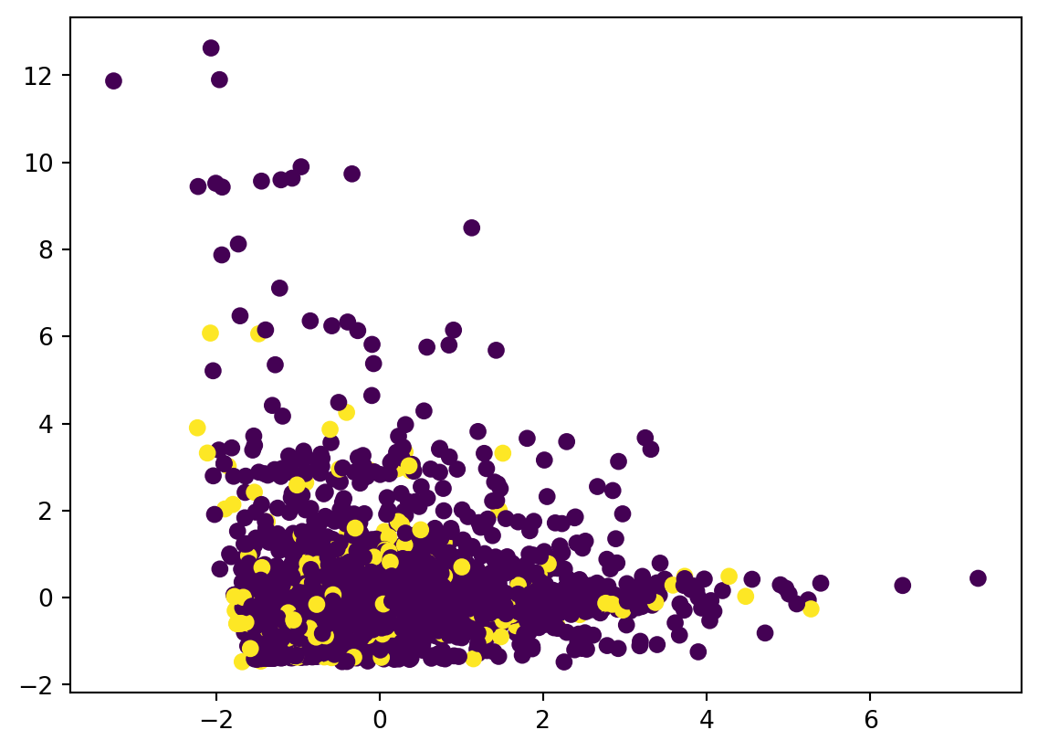

with `4` clusters

km = KMeans(n_clusters=2, max_iter=300, random_state=None)
df_clustering_std['cluster'] = km.fit_predict(df_clustering_std[features_to_explore])

pca = decomposition.PCA(n_components=2, whiten=True)
pca_results = pca.fit_transform(df_clustering_std[features_to_explore])

df_clustering_std['x'] = pca_results[:,0]
df_clustering_std['y'] = pca_results[:,1]

plt.scatter(df_clustering_std['x'], df_clustering_std['y'], c=df_clustering_std['cluster'])
plt.show()

Optimal Number of Clusers

Two find the optimal number of clusters we can user below two methods:

Elbow Method
Silhouette Coefficient

Elbow Method

from sklearn.cluster import KMeans

Sum_of_squared_distances = []

# Use k from 1 to 15
K = range(2,10)
for k in K:
    km = KMeans(n_clusters=k, max_iter=300, random_state=None)
    km = km.fit(df_clustering_std[features_to_explore])
    # Get sum of square distances by applying km.inertia_ 
    Sum_of_squared_distances.append(km.inertia_)

# Plot Results
plt.plot(K, Sum_of_squared_distances, marker='o')
plt.xlabel('k')
plt.ylabel('Sum_of_squared_distances')
plt.title('Elbow Method For Optimal k')
plt.show()

From the elbow we can say that the optimal number of clusters are most likely the 6. The curve decreases strongly from \(k = 2\) to \(k = 6\), meaning each additional cluster gives a meaningful improvement. After \(k = 6\), the decrease becomes much smaller and flatter, so adding more clusters gives only limited extra benefit. That point is the “elbow,” where improvement starts slowing down.

Silhouette Coefficient

from sklearn.metrics import silhouette_samples,silhouette_score

for n_cluster in range(2, 11):
    kmeans = KMeans(n_clusters=n_cluster).fit(df_clustering_std[features_to_explore])
    label = kmeans.labels_
    sil_coeff = silhouette_score(df_clustering_std[features_to_explore], label, metric='euclidean')
    print("For n_clusters={}, The Silhouette Coefficient is {}".format(n_cluster, sil_coeff))

For n_clusters=2, The Silhouette Coefficient is 0.7012956947526441
For n_clusters=3, The Silhouette Coefficient is 0.24990718237250678
For n_clusters=4, The Silhouette Coefficient is 0.26405335168674987
For n_clusters=5, The Silhouette Coefficient is 0.25176450237685666
For n_clusters=6, The Silhouette Coefficient is 0.2729099044337999
For n_clusters=7, The Silhouette Coefficient is 0.15348811540236773
For n_clusters=8, The Silhouette Coefficient is 0.1613343232209698
For n_clusters=9, The Silhouette Coefficient is 0.17235250026465657
For n_clusters=10, The Silhouette Coefficient is 0.16996664692148394

Which is the optimal number?

Profiling the Segments

Let’s stick with the 3 clusters

km = KMeans(n_clusters=3, max_iter=300, random_state=None)
df_clustering_std['cluster'] = km.fit_predict(df_clustering_std[features_to_explore])

pca = decomposition.PCA(n_components=2, whiten=True)
pca_results = pca.fit_transform(df_clustering_std[features_to_explore])

df_clustering_std['x'] = pca_results[:,0]
df_clustering_std['y'] = pca_results[:,1]

plt.scatter(df_clustering_std['x'], df_clustering_std['y'], c=df_clustering_std['cluster'])
plt.show()

We will merge the two dataframes based on a common column user_location_city

Tthe average characteristics of each cluster.
Each row represents the typical behavior of customers/searches that belong to that cluster.

K-Means groups observations around cluster centers, also called centroids. Therefore, these values can be interpreted as the average profile of each cluster.

df_clustering.merge(df_clustering_std[['user_location_city', 'cluster']]).groupby('cluster').mean() # for every column

	duration	days_in_advance	orig_destination_distance	is_mobile	is_package	srch_adults_cnt	srch_children_cnt	srch_rm_cnt	user_location_city
cluster
0	3.186858	52.280953	1808.393230	0.138724	0.235388	2.029434	0.354140	1.097746	28010.250484
1	3.245902	57.950413	1566.755311	0.106557	0.204918	3.905738	0.524590	2.311475	30436.614754
2	4.491226	87.410646	3416.922306	0.125294	0.348193	2.047072	0.339886	1.103835	28058.387789

Summary of Clusters

Cluster	Suggested Name	Main Interpretation
0	Shorter nearby trips	Shorter duration, shorter planning window, lower package usage
1	Long-distance early planners	Farthest destinations and longest booking window
2	Package-oriented travelers	Highest package usage and relatively longer trips

Cluster 0: Shorter Nearby Trips

Cluster 0 represents customers who usually take shorter trips and book relatively closer to the travel date.

Main characteristics:

Average trip duration is around 3.17 days
Average booking window is around 52 days in advance
Average destination distance is around 1,813
Package usage is around 22.5%
Mobile usage is around 13.7%

This cluster can be interpreted as customers who are planning shorter and relatively closer trips. They are less likely to book travel packages compared with Cluster 2.

Cluster 1: Long-Distance Early Planners

Cluster 1 represents customers who travel the longest distances and plan their trips earlier.

Main characteristics:

Average trip duration is around 4.27 days
Average booking window is around 89 days in advance
Average destination distance is around 4,816
Package usage is around 19.4%
Mobile usage is around 10.3%

This cluster can be interpreted as customers who plan long-distance trips well in advance. They are not strongly package-oriented, but their travel distance and planning horizon clearly separate them from the other clusters.

Cluster 2: Package-Oriented Travelers

Cluster 2 represents customers who are much more likely to book package deals.

Main characteristics:

Average trip duration is around 4.33 days
Average booking window is around 74 days in advance
Average destination distance is around 1,936
Package usage is around 50.5%
Mobile usage is around 15.6%

This cluster can be interpreted as customers who prefer package-based travel. They stay slightly longer on average and plan moderately in advance.

Key Differences Between Clusters

The strongest differences between the clusters are observed in:

orig_destination_distance
days_in_advance
is_package
duration

The variables below do not strongly differentiate the clusters because their averages are very similar:

srch_adults_cnt
srch_children_cnt
srch_rm_cnt

The clustering mainly separates customers based on travel distance, planning behavior, and package preference.

Cluster 0: shorter, closer, mostly non-package trips.
Cluster 1: long-distance travelers who book far in advance.
Cluster 2: package-oriented travelers with relatively longer stays.

Overall, Cluster 1 is mainly defined by distance and early planning, while Cluster 2 is mainly defined by package usage.

df_clustering_std['cluster'].unique()

array([0, 2, 1], dtype=int32)

# Plot our Cluster Counts
df_clustering_std.groupby('cluster')['user_location_city'].agg('count').plot(kind='bar')

Learning objectives

Customer Segmentation

Why Segment Customers?

Clustering

Similarity and Distance

Euclidean distance

Manhattan distance

Pearson correlation distance:

Performance of Clustering Algorithms

Clustering Set-Up

K-Means Clustering

K-Means Steps

With Fake Data

Fake Data

K-Means Fit

Optimal Number of Clusters

Elbow Method

Silhouette Analysis

Other Clusering Methods

Hierarchical Clustering

Steps

Intuition

DBSCAN

How it works?

Case Study

Clusering Travel Agency Booking Data

Downloading The Data

Feature Descritpion

Dataframe Size

Information About df

Missing Values

Correlation Matrix

Distributions

is_booking

Merge with the Original Data

Logical Check

Available Travelers

Dates

Feature Enrichment

Statistical Analysis of Booking Channels

Clustering

Feature Selection

Standardize our Data

What Standardization Does

K-means Clustering

Principal Component Analysis (PCA)

with 2 clusters

with 4 clusters

Optimal Number of Clusers

Elbow Method

Silhouette Coefficient

Profiling the Segments

Summary of Clusters

Cluster 0: Shorter Nearby Trips

Cluster 1: Long-Distance Early Planners

Cluster 2: Package-Oriented Travelers

Key Differences Between Clusters

Extra Reading

`is_booking`

with `2` clusters

with `4` clusters