import numpy as np
import pandas as pd

from itertools import combinations

rng = np.random.default_rng(42)

df_sampling = pd.DataFrame(
    {
        "user_id": np.arange(1, 101),
        "category": rng.choice(["A", "B", "C"], size=100, p=[0.5, 0.3, 0.2]),
        "score": rng.normal(loc=75, scale=10, size=100).round(2),
    }
)Session 10: A/B Testing
Multivariate Analysis
Biviate Analysis
Hypothesis Testing
Statistics
Design of Experiments
Outline
In this session we will cover the following topics:
- What is A/B testing?
- A/B testing steps
- Statistics Review
- Hypothesis testing with Python
- Multivariate testing
Tip
Before you start, make sure to read the Statistics Session 6 materials, as we will be using the concepts of hypothesis testing and p-value in this session.
What is A/B Testing?
A/B Testing is a simplified term for randomized controlled experiment, where two samples (A and B) of a single object (product/service) are compared.
Have you ever seen the same website with multiple designs during a certain period of time?

Applications of A/B Testing
- User Experience (UX): Testing Software Navigation, Color, Shape of the components
- Marketing: Testing the content of a campaign
- Drug Development: measuring the effect of the drug compared with either its competitors or placebo
\[\downarrow\]
practically everywhere
Important
In order to give an answer, we need to run an experiment!
Remember the Zen of Python: “In the face of ambiguity, refuse the temptaticon to guess.”
A/B Testing Steps
In general, A/B testing is done with four sequential steps:
- Choose and characterize metrics to evaluate your experiments:
- What do you care about?
- How do you want to measure the effect?
- Power Analysis:
- Significance level (\(\alpha\))
- Statistical power (\(1-\beta\))
- Practical Significance level
- Calculate the required sample size
- Sample for control/treatment groups and run the test
- Analyze the results and draw valid conclusions
Choosing metrics | Step 1
We have two types of metrics:
- Invariant metrics - do not change from control to treatment groups
- Evaluation metrics - the ones in the change of which we are interested.
Four categories of metrics:
- Sums and counts
- Distribution (mean, median, percentiles)
- Probability and rates (e.g. Click-through probability, Click-through rate)
- Ratios: Return on Investment (RoI)
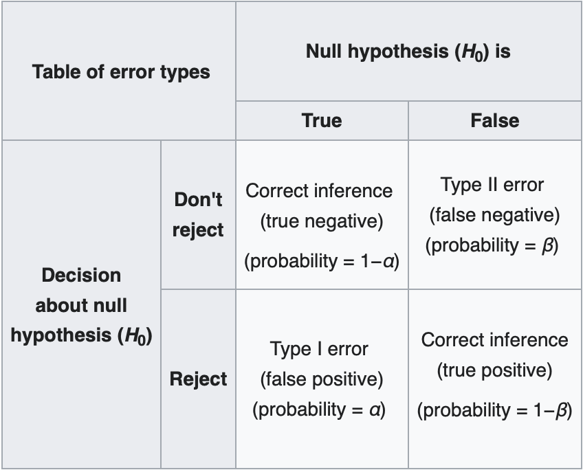
Power Analysis | Step 2
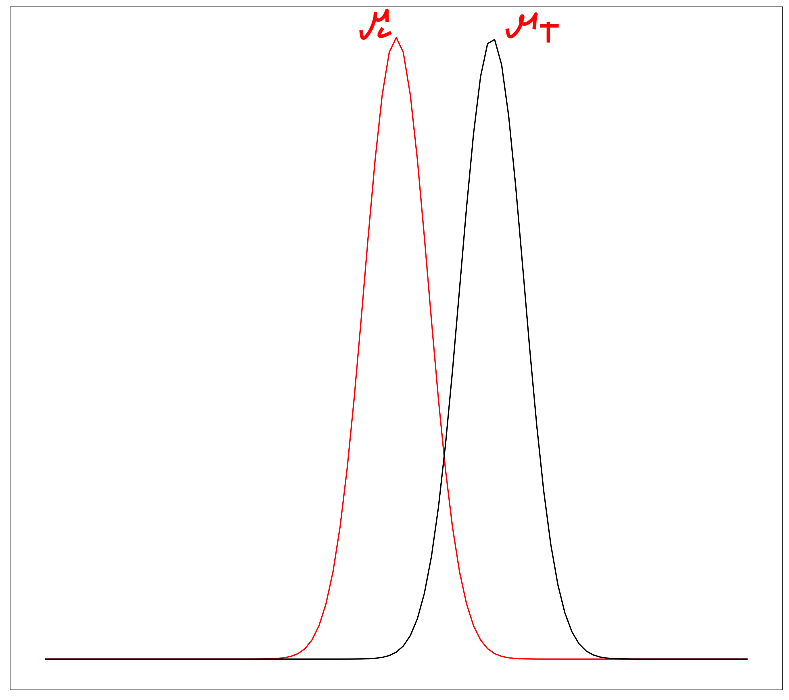
The power of the test (\(1-\beta\)) is the probability of rejecting the \(H_0\) when it is False.
Statistical Power
We use power to calculate the sample size we need. In general, we have the following parameters:
- Power of the test (\(1-\beta\))
- Significance level (\(\alpha\))
- Effect size (\(\delta\))
- Sample size (\(n\))
Note
If you determine any three, the forth will be calculated and derived naturally
The rule of thumb for \(1-\beta\) is 0.8, which means that we have 80% chance of rejecting the \(H_0\) when it is False.
Effect Size
Effect size:
\[H_0: \mu_1=\mu_2\] \[H_1: \mu_1\ne\mu_2\]
Sometimes we want to reject the \(H_0\) with a certain effect, for example when \(|\mu_1-\mu_2|>\delta\)
Effect size use case
The news broadcasting company is testing whether users stay longer on their website with the new website design. The control group consists of visits to the old website, while the treatment group consists of visits to the new website. The new design will be considered effective if the difference in the average duration of the stay is more than 5.5 minutes; thus \(\mu_t-\mu_c >5.5\), the 5.5 here is the effect.
The effect that we want to detect is 5.5, while the effect size is standardized by the standard deviation: \[d = \frac{|\mu_t-\mu_c|}{\sigma}\]
T-Value
The degree of difference relative to the variation in our data groups.
Large t-values indicate a higher degree of difference between the groups.
P-Value
P-value measures the probability that the results would occur by random chance. Therefore, the smaller the p-value is, the more statistically significant difference there will be between the two groups.
Sample size
Sample size will be determined by the below formula:
\[n= \left( \frac{Z_{1-\alpha/2}+Z_{1-\beta/2}}{Effect \text{ }Size} \right)^2\]
where
- \(Z_{1-\alpha/2}\) is the z-score corresponding to the desired confidence level (e.g., for a 95% confidence level, \(Z_{1-\alpha/2} \approx 1.96\))
- \(Z_{1-\beta/2}\) is the z-score corresponding to the desired power level (e.g., for 80% power, \(Z_{1-\beta/2} \approx 0.84\))
- \(Effect \text{ }Size\) is the standardized effect size, calculated as the difference in means divided by the standard deviation.
- \(n\) is the required sample size per group.
Random Sampling | Step 3
Once we have determined the required sample size, we can randomly assign users to either the control or treatment group.
This randomization helps to ensure that any differences observed between the groups can be attributed to the treatment effect rather than confounding variables.
Let’s say we have the following DataFrame:
print(f'The shape of the Dataframe: {df_sampling.shape}' )
print(f'The columns of the Dataframe: {df_sampling.columns}' )
df_sampling.head()
The shape of the Dataframe: (100, 3)
The columns of the Dataframe: Index(['user_id', 'category', 'score'], dtype='str')| user_id | category | score | |
|---|---|---|---|
| 0 | 1 | B | 79.00 |
| 1 | 2 | A | 65.95 |
| 2 | 3 | C | 71.22 |
| 3 | 4 | B | 87.99 |
| 4 | 5 | A | 71.44 |
Summary statistics of the score column:
df_sampling['score'].describe()[['mean', 'std', 'min', 'max']]mean 74.859800
std 9.843752
min 53.680000
max 104.140000
Name: score, dtype: float64df_sampling['category'].value_counts().sort_index()category
A 53
B 33
C 14
Name: count, dtype: int64df_sampling.groupby('category')['score'].describe()[['mean', 'std', 'min', 'max']]| mean | std | min | max | |
|---|---|---|---|---|
| category | ||||
| A | 74.200000 | 8.973076 | 60.29 | 94.97 |
| B | 76.272424 | 10.014058 | 58.25 | 96.28 |
| C | 74.027857 | 12.705514 | 53.68 | 104.14 |
Random Sampling
Suppose we want to take a random sample of 20 users from this DataFrame for our A/B test. We can use the sample method from pandas to do this:
random_sample = df_sampling.sample(n=20, random_state=42)
random_sample.shape
(20, 3)random_sample.groupby('category')['score'].describe()[['mean', 'std', 'min', 'max']]| mean | std | min | max | |
|---|---|---|---|---|
| category | ||||
| A | 71.211250 | 8.747513 | 61.23 | 83.40 |
| B | 75.071429 | 6.553916 | 64.64 | 83.38 |
| C | 67.838000 | 10.015841 | 53.68 | 77.68 |
random_sample['category'].value_counts().sort_index()category
A 8
B 7
C 5
Name: count, dtype: int64Stratified Sampling | proportional to the category distribution
stratified_sample = (
    df_sampling
    .groupby("category", group_keys=False)
    .sample(frac=0.2, random_state=42)
    .reset_index(drop=True)
)
ImportantLine by line explanation
.groupby("category", group_keys=False)- Splits data into strata (A, B, C…)
- Each group is processed independently
.sample(frac=0.2, random_state=42)- Takes 20% from each category
- Preserves distribution
- Deterministic due to seed
stratified_sample.head()| user_id | category | score | |
|---|---|---|---|
| 0 | 39 | A | 78.14 |
| 1 | 84 | A | 77.19 |
| 2 | 93 | A | 92.24 |
| 3 | 29 | A | 89.63 |
| 4 | 86 | A | 86.06 |
Summary statistics of the score column for the stratified sample:
stratified_sample.groupby('category')['score'].describe()[['mean', 'std', 'min', 'max']]| mean | std | min | max | |
|---|---|---|---|---|
| category | ||||
| A | 76.688182 | 10.510287 | 60.29 | 92.24 |
| B | 78.715714 | 10.081969 | 66.79 | 92.68 |
| C | 63.650000 | 5.447054 | 57.73 | 68.45 |
stratified_sample['category'].value_counts().sort_index()category
A 11
B 7
C 3
Name: count, dtype: int64Checking the distribution of the category column in the original DataFrame and the stratified sample:
Original DataFrame category distribution:
df_sampling['category'].value_counts(normalize=True).sort_index()category
A 0.53
B 0.33
C 0.14
Name: proportion, dtype: float64Stratified Sample category distribution:
stratified_sample['category'].value_counts(normalize=True).sort_index()category
A 0.523810
B 0.333333
C 0.142857
Name: proportion, dtype: float64Stratified Sampling | Equal number of samples from each category
There might be situations where we want to ensure an equal number of samples from each category.
stratified_sample = (
    df_sampling
    .groupby("category", group_keys=False)
    .sample(n=10, random_state=42)
    .reset_index(drop=True)
)
Important
n must be less than or equal to the smallest group size in the original DataFrame. In this case, since category C has only 14 samples, we can sample at most 20 from each category.
df_sampling['category'].value_counts()category
A 53
B 33
C 14
Name: count, dtype: int64Splitting the data into control and treatment groups
Pure Random Splitting
- Completely random
- Does NOT preserve category distribution
- Can introduce bias
rng = np.random.default_rng(42)

df_random_split = df_sampling.assign(
    group=rng.choice(["control", "treatment"], size=len(df_sampling))
)df_random_split['group'].value_counts()group
treatment 52
control 48
Name: count, dtype: int64Stratified Splitting
df_stratified_split = (
    df_sampling
    .assign(
        group=lambda x: (
            x.groupby("category")["user_id"]
            .transform(
                lambda g: rng.permutation(
                    ["control"] * (len(g)//2) +
                    ["treatment"] * (len(g) - len(g)//2)
                )
            )
        )
    )
)df_stratified_split[['group', 'category']].value_counts()group category
treatment A 27
control A 26
treatment B 17
control B 16
treatment C 7
control C 7
Name: count, dtype: int64Analyzing the results | Step 4
Recall the decision rules for hypothesis testing fro Statistics Session 6:
See
- @materials/statistics/session6.qmd#sec-hypothesis-testing-decision-rules
- @materials/statistics/session6.qmdsec-visual-representation-hypothesis-testing
A/B Testing With Python
Loading Packages
import numpy as np
import pandas as pd
import math
from statsmodels.stats.power import TTestIndPower
from statsmodels.stats.multitest import multipletests
from scipy.stats import ttest_ind
import scipy
import matplotlib.pyplot as plt
Tip
Do not forget to install the required packages before running the code.
Make sure that you are in the correct virtual environment, and run the following command in your terminal:
bash
pip install statsmodels scipy
NOTE: you must run the above command in your terminal, given the fact that the your virtual environment is activated.
Calculating Sample Size
How much sample do you need to take, if you want to detect effect size of \(0.4\), with the power of \(0.8\) and significance level of \(0.05\) ?
You will do two independent samples t-test.
N = TTestIndPower().solve_power(effect_size = 0.4, power = 0.8,
                            alpha = 0.05)

N99.08032514659006Note, sample size is per group 100
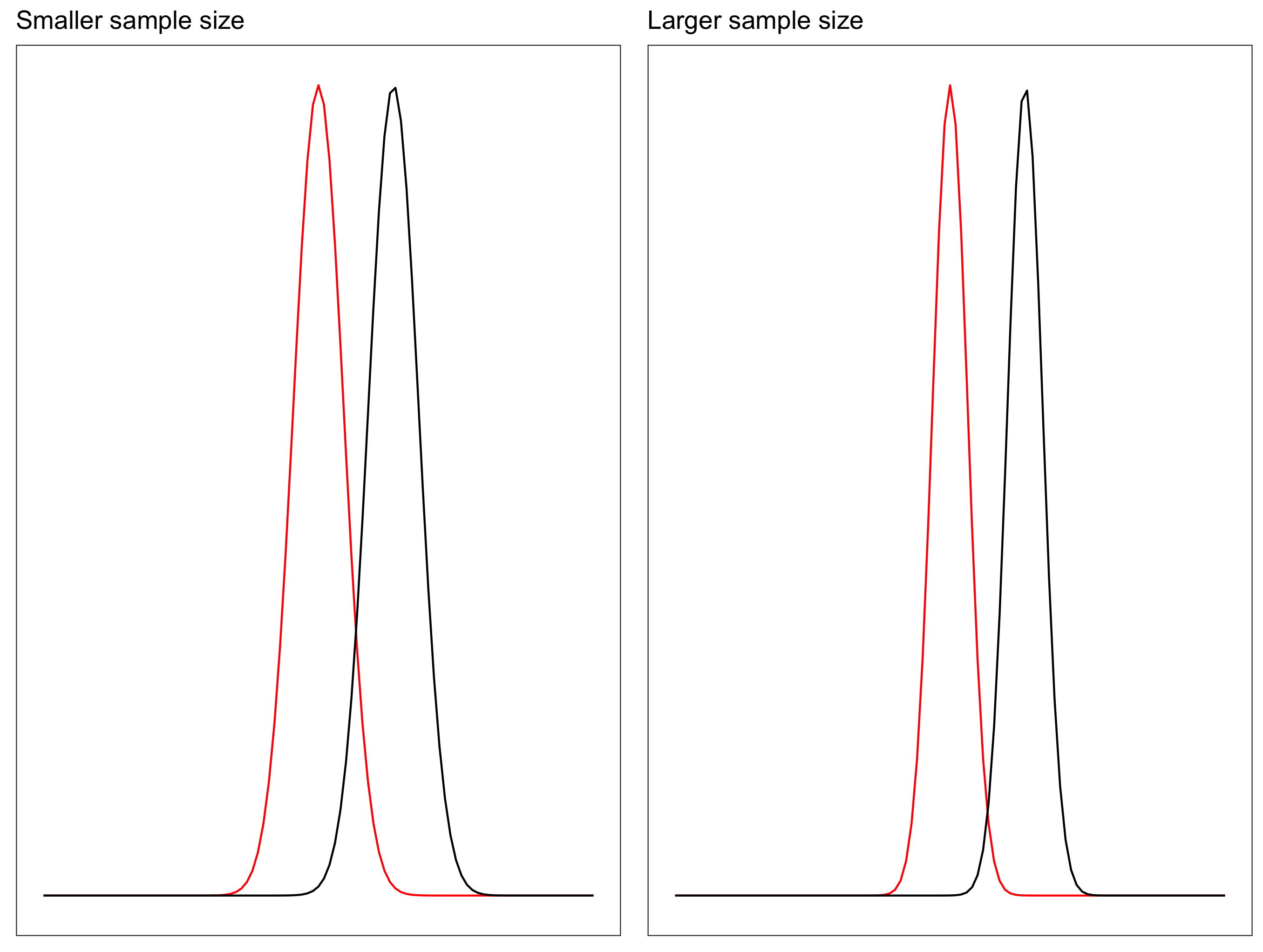
Sampling distributions
Sampling distribution of the means for two groups (control and treatment):
\[H_0: \mu_c=\mu_t\] \[H_1: \mu_c\ne\mu_t\]
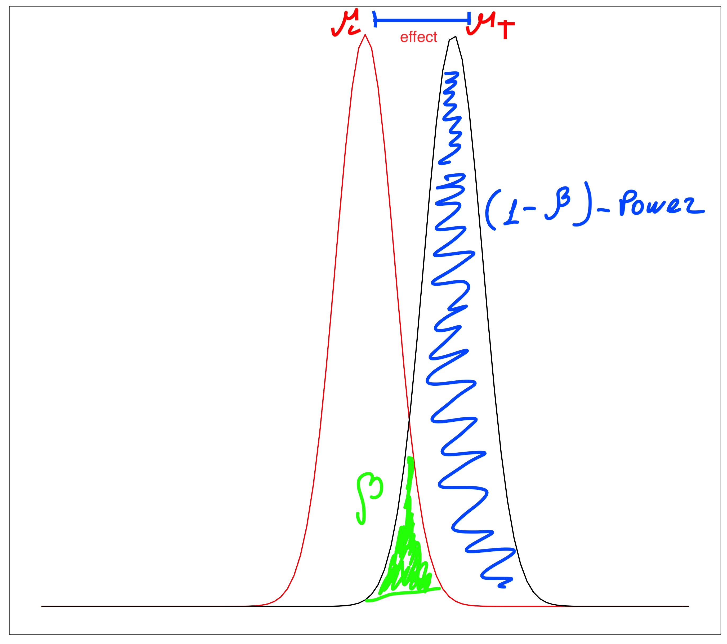
Power
Relationship between power and effect size: There is a direct relationship between power and effect size: Increasing the effect size will increase power.
TTestIndPower().plot_power(dep_var='nobs',
                            nobs=np.array(range(5, 100)),
                            effect_size=np.array([0.2, 0.5, 0.8]),
                            title='Power of t-Test')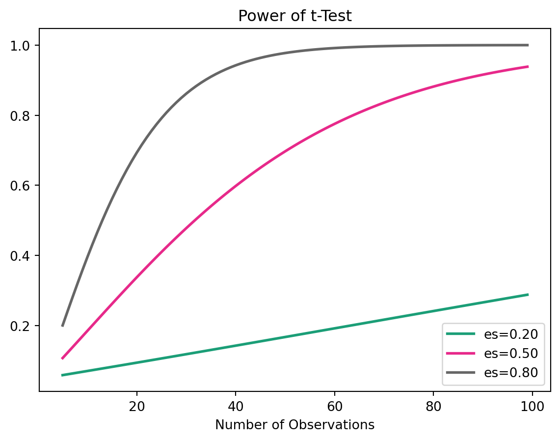

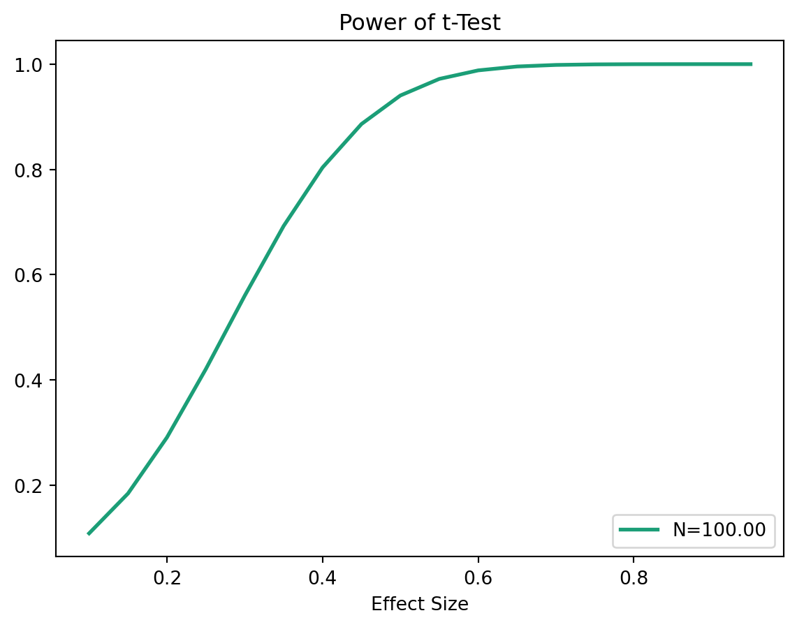
Plot power and effect size using python, sample size = 100
TTestIndPower().plot_power(dep_var='effect_size', nobs= [100],
                                 effect_size=np.arange(0.1, 1, 0.05),
                                 title='Power of t-Test')
Increasing sample size will also increase the power, as with the higher sample size the sampling distribution of the mean becomes narrower. Recall, the standard deviation of the sampling distribution (Standard Error) of the mean is calculated as: \[SE = \frac{\sigma}{\sqrt{n}}\]
Hypothesis Testing
TipUse case
The news streaming company is adding a new feature to the website. The effect the company is trying to detect is equal to 5 minutes.
- It is a randomized experiment, meaning that every visitor to the site will have 0.5 probability of being in the treatment (new feature) group and 0.5 probability of being in control group (old design).
- The minimum effect they want to detect is an increase by 5 minutes.
- From the historical data they have estimated the standard deviation to be 13.7 minutes.
The hypothesis:
\[H_0: \mu_t = \mu_c\] \[H_1: \mu_t\ne\mu_c\]
Sample Size
Specifications:
- \(\sigma = 13.7\)
- Power: \((1-\beta) = 0.8\)
- Significance level: \(\alpha = 0.05\)
- Effect size: \(\frac{|\mu_t-\mu_c|}{\sigma} = \frac{5}{13.7} = 0.365\)
Determine the sample size for each group:
TTestIndPower().solve_power(effect_size = 0.365, power = 0.8,
alpha = 0.05, alternative = 'larger')93.49756951363241Loading the data
Load the data
| user_id | viewing_time | Group | |
|---|---|---|---|
| 0 | 4b5630ee914e848e8d07221556b0a2fb | 38.354937 | control |
| 1 | c01f179e4b57ab8bd9de309e6d576c48 | 49.534278 | control |
| 2 | 11946e7a3ed5e1776e81c0f0ecd383d0 | 35.468325 | control |
| 3 | 234a2a5581872457b9fe1187d1616b13 | 69.014875 | control |
| 4 | dd4ad37ee474732a009111e3456e7ed7 | 51.547207 | control |
expr = pd.read_csv('../data/ab_testing/experiment.csv')
expr.head()expr.groupby('Group')['viewing_time'].mean()Group
control 48.386186
treatment 52.081302
Name: viewing_time, dtype: float64T-test
T-test with scipy:
ctrl = expr[expr['Group'] == 'control']['viewing_time']
treatment = expr[expr['Group'] == 'treatment']['viewing_time']
test_res = ttest_ind(treatment, ctrl)
tstat, pvalue=test_resf"t-statistics: {tstat:.4f}"'t-statistics: 1.6002'f"p-value: {pvalue:.4f}"'p-value: 0.1128'Interpretation
We failed to reject the \(H_0\) where \(\alpha = 0.05\). We haven’t seen the anticipated improvement!
How much improvement is there ?
diff=treatment.mean() - ctrl.mean()
sd_pooled=math.sqrt((treatment.std()**2+ ctrl.std()**2)/2)
To find the detected effect size, calculate Cohen’s d.
\[\frac{\bar{x_t}-\bar{x_c}}{pooled \; SD}\]
\[\downarrow\]
\[\frac{\bar{x_t}-\bar{x_c}}{\sqrt{(s_t^2+s_c^2)/2}}\]
f"The detected Effect: {diff/sd_pooled:.4f}"'The detected Effect: 0.3200'Practical Significance
There could be cases, where statistical tests show significnce while in the reality the difference is not that actual.
Such effects might happen in bellow cases:
- low variance between two samples
- the sample size is huge
Recall:
\[t_{value}=\frac{\bar{x_1}-\bar{x_1}}{\sqrt{\frac{s_1^2}{n_1}+\frac{s_2^2}{n_2}}}\]
Utils Functions
First, lets define some helper functions to compute the t-statistic and p-value for two independent samples.
The function below computes key statistical measures from a dataset and extracts:
- Mean of
score1 - Mean of
score2 - Standard deviation of
score1 - Standard deviation of
score2
def measures(data):
    desc = data.describe()
    x1 = desc.loc['mean', 'score1']
    x2 = desc.loc['mean', 'score2']
    s1 = desc.loc['std', 'score1']
    s2 = desc.loc['std', 'score2']
    return x1, x2, s1, s2
The Function below computes the t-value and p-value for two independent samples using the formula for the t-statistic and the survival function from the scipy.stats module to calculate the p-value.
def ttest(x1,x2,s1,s2,n):
    t_value = (x1-x2)/math.sqrt(s1**2/n+s2**2/n)
    p_value = scipy.stats.t.sf(abs(t_value), df=n-1)*2
    return f't-value: {t_value:.4f}', f'p-value: {p_value:.4f}'
Case 1 | low variance
case1=pd.read_csv("../data/ab_testing/case1.csv")
case1.head()| score1 | score2 | |
|---|---|---|
| 0 | 85 | 87 |
| 1 | 85 | 86 |
| 2 | 86 | 87 |
| 3 | 86 | 86 |
| 4 | 85 | 86 |
case1.describe().loc[['count','mean','std']]| score1 | score2 | |
|---|---|---|
| count | 20.000000 | 20.000000 |
| mean | 85.550000 | 86.400000 |
| std | 0.510418 | 0.502625 |
Experiment
# t-test for case 1
c1=measures(case1)
ttest(*c1,20)
('t-value: -5.3065', 'p-value: 0.0000')
Important
However, the t-test shows that there is a significant difference between the two groups, with a t-value of 2.8284 and a p-value of 0.0050. This is because the low variance in the data makes it easier to detect even small differences between the groups, leading to a statistically significant result.
Case 2 | huge sample size
case2=pd.read_csv("../data/ab_testing/case2.csv")
case2.head()| score1 | score2 | |
|---|---|---|
| 0 | 88 | 95 |
| 1 | 89 | 88 |
| 2 | 91 | 93 |
| 3 | 94 | 87 |
| 4 | 87 | 89 |
case2.describe().loc[['count','mean','std']]| score1 | score2 | |
|---|---|---|
| count | 20.000000 | 20.000000 |
| mean | 90.650000 | 90.750000 |
| std | 2.777257 | 2.788605 |
Experiment
Now we will apply the t-test to case 2, which has a huge sample size of 20,000, however at first will will start with smaller sample size to see how the results change with the increase of the sample size.
N=200
c2=measures(case2)
ttest(*c2,200)
('t-value: -0.3593', 'p-value: 0.7197')N=200
c2=measures(case2)
ttest(*c2,200)
('t-value: -0.3593', 'p-value: 0.7197')N=2000
c2=measures(case2)
ttest(*c2,2000)
('t-value: -1.1363', 'p-value: 0.2560')N=20000
c2=measures(case2)
ttest(*c2,20000)
('t-value: -3.5933', 'p-value: 0.0003')
Important
As we can see, as the sample size increases, the t-value increases and the p-value decreases, leading to a statistically significant result. This is because with a huge sample size, even very small differences between the groups can become statistically significant, which may not be practically significant in real-world terms.
A/A Testing
A/A testing is a type of experiment where two identical versions of a product or service are compared to each other. The purpose of A/A testing is to validate the experimental setup and ensure that there are no biases or confounding factors that could affect the results of future A/B tests.

Multiariate Testing
In real life, we often have more than two groups to compare. For example, we might want to test multiple versions of a website design or several different marketing campaigns.

Infinite Monkey Theorem
The Infinite Monkey Theorem says that if random typing continues for long enough, even very unlikely strings will eventually appear.
This is a useful analogy for hypothesis testing.
- when we run one test, the probability of a false positive is controlled at \(\alpha\)
- when we run many tests, the chance of seeing at least one false positive increases
- so, with enough tests, some apparently significant results may appear purely by chance

Why multiple testing is a problem
For a single hypothesis test:
\[P(\text{Type I error}) = \alpha\]
\[P(\text{No Type I error}) = 1 - \alpha\]
If we perform m independent hypothesis tests, then:
\[P(\text{No Type I error in all } m \text{ tests}) = (1-\alpha)^m\]
Therefore, the probability of making at least one Type I error becomes:
\[P(\text{At least one Type I error}) = 1 - (1-\alpha)^m\]
This means that even if each test looks safe on its own, the overall analysis becomes riskier as the number of tests grows.
Type I error means a false positive: rejecting the null hypothesis when it is actually true.
Loading packages
import matplotlib.pyplot as plt
from scipy import stats
from statsmodels.stats.multitest import multipletests
Type I error curve
The following plot shows how quickly the probability of observing at least one false positive grows as the number of hypothesis tests increases when \(\alpha = 0.05\).
m_tests = np.arange(0, 101)
prob_at_least_one_error = 1 - (1 - 0.05) ** m_tests

plt.figure()
plt.plot(m_tests, prob_at_least_one_error)
plt.xlabel("Number of hypotheses")
plt.ylabel("Probability of at least 1 Type I error")
plt.title("Family-level risk grows as the number of tests increases")
plt.show()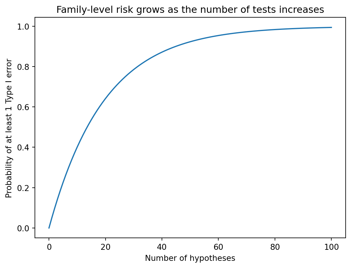
Multiple hypotheses
Assume we are testing \(H^1, H^2, \ldots, H^m\).
- \(m\) is the total number of hypotheses
- \(m_0\) is the number of truly null hypotheses
- \(R\) is the number of rejected hypotheses
- \(V\) is the number of Type I errors among the rejected hypotheses
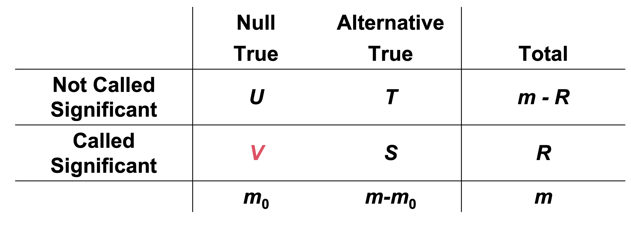
\(V\) is the number of false positives.
Controlling the Type I error
There are several ways to summarize error rates when multiple tests are performed.
Per comparison error rate (PCER): the expected number of Type I errors divided by the number of hypotheses
\[PCER = \mathbb{E}[V]/m\]
Per-family error rate (PFER): the expected number of Type I errors
\[PFER = \mathbb{E}[V]\]
Family-wise error rate (FWER): the probability of making at least one Type I error
\[FWER = P(V \ge 1)\]
False discovery rate (FDR): the expected proportion of Type I errors among the rejected hypotheses
\[FDR = \mathbb{E}\left(\frac{V}{R} \mid R > 0\right) P(R > 0)\]
The main difference is the target being controlled.
- FWER is very strict because it tries to protect against even a single false positive
- FDR is more flexible because it focuses on the proportion of false discoveries among the reported discoveries
Loading the data
We now use the experiment_m.csv data set.
experiment_m = pd.read_csv("../../lab/python/data/ab_testing/experiment_m.csv")
groups = sorted(experiment_m["group"].dropna().unique())
#| echo: true
experiment_m = pd.read_csv("../data/ab_testing/experiment_m.csv")
groups = sorted(experiment_m["group"].dropna().unique())group_counts = (
experiment_m.groupby("group", as_index=False)
.size()
.rename(columns={"size": "n"})
)
group_counts| group | n | |
|---|---|---|
| 0 | Test1 | 200 |
| 1 | Test2 | 200 |
| 2 | Test3 | 200 |
| 3 | Test4 | 200 |
| 4 | Test5 | 200 |
| 5 | Test6 | 200 |
| 6 | Test7 | 200 |
| 7 | Test8 | 200 |
| 8 | Test9 | 200 |
| 9 | control | 200 |
| group | n |
|---|---|
| Test1 | 200 |
| Test2 | 200 |
| Test3 | 200 |
| Test4 | 200 |
| Test5 | 200 |
| Test6 | 200 |
| Test7 | 200 |
| Test8 | 200 |
| Test9 | 200 |
| control | 200 |
This table helps us verify the sample size in each group before starting the pairwise tests.
Pairwise t-test without adjustment
We first compute all pairwise t-tests with no correction.
We use Welch’s t-test rather than the equal-variance version because this matches the logic of the original R code with pooled.sd = FALSE.
pairwise_results = pairwise_ttests(
    experiment_m,
    value_col="viewing_time",
    group_col="group"
)

pairwise_results.head()| group_1 | group_2 | t_statistic | raw_p_value | |
|---|---|---|---|---|
| 0 | Test1 | Test2 | -2.845693 | 0.004686 |
| 1 | Test1 | Test3 | -1.917291 | 0.055942 |
| 2 | Test1 | Test4 | -2.799258 | 0.005391 |
| 3 | Test1 | Test5 | 0.279632 | 0.779907 |
| 4 | Test1 | Test6 | -3.281141 | 0.001125 |
The next table shows the raw pairwise p-values before any adjustment is applied.
| group_1 | group_2 | raw_p_value |
|---|---|---|
| Test6 | Test8 | 0.0000 |
| Test6 | control | 0.0000 |
| Test4 | Test8 | 0.0000 |
| Test2 | Test8 | 0.0000 |
| Test2 | control | 0.0000 |
| Test4 | control | 0.0000 |
| Test3 | Test8 | 0.0002 |
| Test5 | Test6 | 0.0007 |
| Test3 | control | 0.0008 |
| Test1 | Test6 | 0.0011 |
| Test2 | Test5 | 0.0030 |
| Test4 | Test5 | 0.0035 |
| Test6 | Test7 | 0.0044 |
| Test1 | Test2 | 0.0047 |
| Test1 | Test4 | 0.0054 |
| Test8 | Test9 | 0.0087 |
| Test2 | Test7 | 0.0125 |
| Test7 | Test8 | 0.0142 |
| Test4 | Test7 | 0.0147 |
| Test9 | control | 0.0206 |
| Test1 | Test8 | 0.0344 |
| Test7 | control | 0.0361 |
| Test3 | Test5 | 0.0368 |
| Test6 | Test9 | 0.0485 |
| Test1 | Test3 | 0.0559 |
| Test2 | Test9 | 0.0669 |
| Test1 | control | 0.0768 |
| Test5 | Test8 | 0.0777 |
| Test4 | Test9 | 0.0799 |
| Test3 | Test7 | 0.1209 |
| Test5 | control | 0.1476 |
| Test5 | Test9 | 0.2979 |
| Test3 | Test6 | 0.2982 |
| Test2 | Test3 | 0.3059 |
| Test3 | Test9 | 0.3601 |
| Test3 | Test4 | 0.3605 |
| Test1 | Test9 | 0.4072 |
| Test5 | Test7 | 0.5215 |
| Test7 | Test9 | 0.6211 |
| Test1 | Test7 | 0.7021 |
| Test1 | Test5 | 0.7799 |
| Test8 | control | 0.8067 |
| Test2 | Test6 | 0.8777 |
| Test2 | Test4 | 0.8941 |
| Test4 | Test6 | 0.9960 |
Raw p-value matrix
A matrix view is often easier to scan when many group comparisons are involved.
| index | Test1 | Test2 | Test3 | Test4 | Test5 | Test6 | Test7 | Test8 | Test9 | control |
|---|---|---|---|---|---|---|---|---|---|---|
| Test1 | — | 0.0047 | 0.0559 | 0.0054 | 0.7799 | 0.0011 | 0.7021 | 0.0344 | 0.4072 | 0.0768 |
| Test2 | 0.0047 | — | 0.3059 | 0.8941 | 0.0030 | 0.8777 | 0.0125 | 0.0000 | 0.0669 | 0.0000 |
| Test3 | 0.0559 | 0.3059 | — | 0.3605 | 0.0368 | 0.2982 | 0.1209 | 0.0002 | 0.3601 | 0.0008 |
| Test4 | 0.0054 | 0.8941 | 0.3605 | — | 0.0035 | 0.9960 | 0.0147 | 0.0000 | 0.0799 | 0.0000 |
| Test5 | 0.7799 | 0.0030 | 0.0368 | 0.0035 | — | 0.0007 | 0.5215 | 0.0777 | 0.2979 | 0.1476 |
| Test6 | 0.0011 | 0.8777 | 0.2982 | 0.9960 | 0.0007 | — | 0.0044 | 0.0000 | 0.0485 | 0.0000 |
| Test7 | 0.7021 | 0.0125 | 0.1209 | 0.0147 | 0.5215 | 0.0044 | — | 0.0142 | 0.6211 | 0.0361 |
| Test8 | 0.0344 | 0.0000 | 0.0002 | 0.0000 | 0.0777 | 0.0000 | 0.0142 | — | 0.0087 | 0.8067 |
| Test9 | 0.4072 | 0.0669 | 0.3601 | 0.0799 | 0.2979 | 0.0485 | 0.6211 | 0.0087 | — | 0.0206 |
| control | 0.0768 | 0.0000 | 0.0008 | 0.0000 | 0.1476 | 0.0000 | 0.0361 | 0.8067 | 0.0206 | — |
At this stage, every p-value is interpreted as if it were the only test being performed.
That is exactly why multiple testing corrections are needed.
Case Study | Fast Food Chain
Problem Scenario
Which promotion was the most effective?
A fast food chain plans to add a new item to its menu. However, they are still undecided between three possible marketing campaigns for promoting the new product. In order to determine which promotion has the greatest effect on sales, the new item is introduced at locations in several randomly selected markets. A different promotion is used at each location, and the** weekly sales** of the new item are recorded for the first four weeks
The description of the data set:
The data set consists of 548 entries including:
- MarketId: an inhouse tag used to describe market types, we won’t be using it
- AgeOfStores: Age of store in years (1–28). The mean age of a store is 8.5 years.
- LocationID: Unique identifier for store location. Each location is identified by a number. The total number of stores is 137.
- Promotion: One of three promotions that were tested (1, 2, 3). We don’t really know the specifics of each promotion.
- Sales in Thousands: Sales amount for a specific LocationID, Promotion and week. The mean amount of sales are 53.5 thousand dollars.
- Market size: there are three types of market size: small, medium and large.
- Week: One of four weeks when the promotions were run (1–4).
Importing Data and Libraries
import pandas as pddf = pd.read_csv('../data/ab_testing/fast_food.csv')
df.head()| MarketID | MarketSize | LocationID | AgeOfStore | Promotion | week | SalesInThousands | |
|---|---|---|---|---|---|---|---|
| 0 | 1 | Medium | 1 | 4 | 3 | 1 | 33.73 |
| 1 | 1 | Medium | 1 | 4 | 3 | 2 | 35.67 |
| 2 | 1 | Medium | 1 | 4 | 3 | 3 | 29.03 |
| 3 | 1 | Medium | 1 | 4 | 3 | 4 | 39.25 |
| 4 | 1 | Medium | 2 | 5 | 2 | 1 | 27.81 |
print(f"""
Rows           : {df.shape[0]}
Columns        : {df.shape[1]}

Features       :
{df.columns.tolist()}

Missing values : {df.isnull().sum().sum()}

Unique values  :
{df.nunique()}
""")
Rows           : 548
Columns        : 7

Features       :
['MarketID', 'MarketSize', 'LocationID', 'AgeOfStore', 'Promotion', 'week', 'SalesInThousands']

Missing values : 0

Unique values  :
MarketID             10
MarketSize            3
LocationID          137
AgeOfStore           25
Promotion             3
week                  4
SalesInThousands    517
dtype: int64
df.describe()| MarketID | LocationID | AgeOfStore | Promotion | week | SalesInThousands | |
|---|---|---|---|---|---|---|
| count | 548.000000 | 548.000000 | 548.000000 | 548.000000 | 548.000000 | 548.000000 |
| mean | 5.715328 | 479.656934 | 8.503650 | 2.029197 | 2.500000 | 53.466204 |
| std | 2.877001 | 287.973679 | 6.638345 | 0.810729 | 1.119055 | 16.755216 |
| min | 1.000000 | 1.000000 | 1.000000 | 1.000000 | 1.000000 | 17.340000 |
| 25% | 3.000000 | 216.000000 | 4.000000 | 1.000000 | 1.750000 | 42.545000 |
| 50% | 6.000000 | 504.000000 | 7.000000 | 2.000000 | 2.500000 | 50.200000 |
| 75% | 8.000000 | 708.000000 | 12.000000 | 3.000000 | 3.250000 | 60.477500 |
| max | 10.000000 | 920.000000 | 28.000000 | 3.000000 | 4.000000 | 99.650000 |
Exploratory Data Analysis (EDA)
Sales Distribution by Promotion
Instead of total sales (which can be biased), we look at distribution
fig = px.box(
    df,
    x="Promotion",
    y="SalesInThousands",
    color="Promotion",
    title="Sales Distribution by Promotion"
)
fig.show()
Average Sales per Promotion
promo_avg = (
    df.groupby("Promotion")["SalesInThousands"]
    .mean()
    .reset_index()
)

fig = px.bar(
    promo_avg,
    x="Promotion",
    y="SalesInThousands",
    text="SalesInThousands",
    title="Average Sales by Promotion"
)
fig.show()
Sales Trend Over Time
weekly_sales = (
    df.groupby(["week", "Promotion"])["SalesInThousands"]
    .mean()
    .reset_index()
)

fig = px.line(
    weekly_sales,
    x="week",
    y="SalesInThousands",
    color="Promotion",
    markers=True,
    title="Weekly Sales Trend by Promotion"
)
fig.show()
A promotion might look good overall but fade over time.
Market Size Effect
fig = px.box(
    df,
    x="MarketSize",
    y="SalesInThousands",
    color="Promotion",
    title="Sales by Market Size and Promotion"
)
fig.show()
Store Age Impact
fig = px.scatter(
    df,
    x="AgeOfStore",
    y="SalesInThousands",
    color="Promotion",
    trendline="ols",
    title="Sales vs Store Age"
)
fig.show()
Statistical Testing
Aggregating the date per Store
# better: aggregate per store first
store_level = (
    df.groupby(["LocationID", "Promotion"])["SalesInThousands"]
    .mean()
    .reset_index()
)
Comparing Promotion 1 vs Promotion 2 in an A/B Test
t,p = stats.ttest_ind(
    store_level[store_level["Promotion"] == 1]["SalesInThousands"],
    store_level[store_level["Promotion"] == 2]["SalesInThousands"],
    equal_var=False
)

print(f"T-statistic: {t:.4f}, P-value: {p:.4f}")
T-statistic: 3.3321, P-value: 0.0013The p-value is less than 0.05, so we reject the null hypothesis and conclude that there is a statistically significant difference in sales between Promotion 1 and Promotion 2.
Comparing Promotion 1 vs Promotion 3
t, p = stats.ttest_ind(
    df.loc[df['Promotion'] == 1, 'SalesInThousands'].values,
    df.loc[df['Promotion'] == 3, 'SalesInThousands'].values,
    equal_var=False)

print("t-value = " +str(t))
print("p-value = " +str(p))
t-value = 1.5560224307758634
p-value = 0.12059147742229478The p-value is greater than 0.05, so we fail to reject the null hypothesis and conclude that there is no statistically significant difference in sales between Promotion 1 and Promotion 3.