import os
import zipfile
import requests
import numpy as np
import pandas as pd
import plotly.express as px
import folium

from tqdm import tqdm
from pathlib import PathSession 15: Geoanalytics
Geoanalytics
Folium
KaplerGl
Session Goal
In this session, we move from classical data analysis to geospatial analytics.
Instead of analyzing only what happened and when it happened, we also analyze where it happened.
We will use Citi Bike trip data as a real-world case study.
By the end of this session, students will be able to:
- understand basic geographic vocabulary
- work with latitude and longitude
- download real-world trip data
- clean and aggregate large datasets
- create station-level and route-level summaries
- apply stratified sampling
- test whether sample-based insights are stable
- visualize geographic patterns using Folium and Kepler.gl
The official Citi Bike system data page publishes downloadable trip history files, including ride ID, ride type, start and end times, station names, station IDs, coordinates, and membership type.
The data is available through the Citi Bike system data page and public trip-data bucket.
Why Geospatial Analytics?
Traditional analysis usually answers questions like:
- how many rides happened?
- when did rides happen?
- which customer type used the service more?
- how did volume change by month?
Geospatial analysis adds another layer:
- where did rides start?
- where did rides end?
- which stations are most active?
- which areas are connected by frequent trips?
- how does movement change by season?
In simple terms:
Geospatial analytics connects data with location.
For Citi Bike, every ride has both a time dimension and a location dimension.
| Dimension | Example Columns | Analytical Question |
|---|---|---|
| Time | started_at, ended_at |
When do people ride? |
| Location | start_lat, start_lng, end_lat, end_lng |
Where do rides happen? |
| Station | start_station_name, end_station_name |
Which stations are important? |
| User Type | member_casual |
Who uses the service? |
| Bike Type | rideable_type |
What type of bike is used? |
The full session has two parts:
- Geographic Foundations
- Citi Bike End to End Analysis
Part 1: Geographic Foundations
Before downloading large data, we first understand the geographic building blocks.
We will cover:
- latitude and longitude
- points
- lines
- flows
- bounding boxes
- distance
- spatial aggregation
- station-level summaries
- route-level summaries
Part 2: Citi Bike End-to-End Analysis
Then we move to the real project workflow.
We will:
- install required packages
- create project folders
- download Citi Bike monthly data
- load and clean the data
- aggregate daily and monthly volumes
- create seasonal variables
- build station-level datasets
- build route-level datasets
- create stratified samples
- test different random seeds
- visualize data with Plotly, Folium, and Kepler.gl
- save reusable datasets for future analysis
Installing Required Packages
We will use the following packages.
| Package | Purpose |
|---|---|
folium |
interactive maps |
keplergl |
advanced geospatial visualization |
tqdm |
progress bars |
Install them from the terminal:
pip install pandas numpy requests plotly folium keplergl tqdm
ImportantIn case of error
Install them from the terminal using conda:
conda install pandas numpy requests plotly folium keplergl tqdmImport Libraries
Geographic Foundations
Latitude and Longitude
A geographic location is usually represented by two numbers:
| Term | Meaning |
|---|---|
| Latitude | North-south position |
| Longitude | East-west position |
For example:
| City | Latitude | Longitude |
|---|---|---|
| New York City | 40.7128 | -74.0060 |
| Yerevan | 40.1872 | 44.5152 |
- Latitude: tells us how far north or south a point is
- Longitude tells us how far east or west a point is.
Demo Trip DF
trip_demo = pd.DataFrame({
    "ride_id": list(range(1, 21)),

    "start_station": [
        "Station A", "Station A", "Station A", "Station A", "Station A",
        "Station B", "Station B", "Station B", "Station B",
        "Station C", "Station C", "Station C",
        "Station D", "Station D", "Station D",
        "Station E", "Station E",
        "Station A", "Station B", "Station C"
    ],

    "end_station": [
        "Station B", "Station B", "Station B", "Station C", "Station C",
        "Station A", "Station A", "Station C", "Station D",
        "Station A", "Station B", "Station E",
        "Station A", "Station C", "Station E",
        "Station A", "Station D",
        "Station E", "Station E", "Station D"
    ],

    "started_at": pd.to_datetime([
        "2025-01-01 08:00", "2025-01-01 08:15", "2025-01-01 08:30",
        "2025-01-01 09:00", "2025-01-01 09:20",
        "2025-01-01 10:00", "2025-01-01 10:15", "2025-01-01 10:40",
        "2025-01-01 11:00",
        "2025-01-01 11:30", "2025-01-01 12:00", "2025-01-01 12:20",
        "2025-01-01 13:00", "2025-01-01 13:30", "2025-01-01 14:00",
        "2025-01-01 14:30", "2025-01-01 15:00",
        "2025-01-01 15:30", "2025-01-01 16:00", "2025-01-01 16:30"
    ]),

    "ended_at": pd.to_datetime([
        "2025-01-01 08:10", "2025-01-01 08:28", "2025-01-01 08:42",
        "2025-01-01 09:18", "2025-01-01 09:35",
        "2025-01-01 10:12", "2025-01-01 10:30", "2025-01-01 10:55",
        "2025-01-01 11:18",
        "2025-01-01 11:48", "2025-01-01 12:14", "2025-01-01 12:45",
        "2025-01-01 13:20", "2025-01-01 13:48", "2025-01-01 14:20",
        "2025-01-01 14:55", "2025-01-01 15:22",
        "2025-01-01 15:58", "2025-01-01 16:25", "2025-01-01 16:50"
    ]),

    "member_casual": [
        "member", "member", "casual", "member", "casual",
        "member", "member", "casual", "member",
        "casual", "member", "casual",
        "member", "casual", "member",
        "casual", "member",
        "member", "casual", "member"
    ]
})

trip_demo| ride_id | start_station | end_station | started_at | ended_at | member_casual | |
|---|---|---|---|---|---|---|
| 0 | 1 | Station A | Station B | 2025-01-01 08:00:00 | 2025-01-01 08:10:00 | member |
| 1 | 2 | Station A | Station B | 2025-01-01 08:15:00 | 2025-01-01 08:28:00 | member |
| 2 | 3 | Station A | Station B | 2025-01-01 08:30:00 | 2025-01-01 08:42:00 | casual |
| 3 | 4 | Station A | Station C | 2025-01-01 09:00:00 | 2025-01-01 09:18:00 | member |
| 4 | 5 | Station A | Station C | 2025-01-01 09:20:00 | 2025-01-01 09:35:00 | casual |
| 5 | 6 | Station B | Station A | 2025-01-01 10:00:00 | 2025-01-01 10:12:00 | member |
| 6 | 7 | Station B | Station A | 2025-01-01 10:15:00 | 2025-01-01 10:30:00 | member |
| 7 | 8 | Station B | Station C | 2025-01-01 10:40:00 | 2025-01-01 10:55:00 | casual |
| 8 | 9 | Station B | Station D | 2025-01-01 11:00:00 | 2025-01-01 11:18:00 | member |
| 9 | 10 | Station C | Station A | 2025-01-01 11:30:00 | 2025-01-01 11:48:00 | casual |
| 10 | 11 | Station C | Station B | 2025-01-01 12:00:00 | 2025-01-01 12:14:00 | member |
| 11 | 12 | Station C | Station E | 2025-01-01 12:20:00 | 2025-01-01 12:45:00 | casual |
| 12 | 13 | Station D | Station A | 2025-01-01 13:00:00 | 2025-01-01 13:20:00 | member |
| 13 | 14 | Station D | Station C | 2025-01-01 13:30:00 | 2025-01-01 13:48:00 | casual |
| 14 | 15 | Station D | Station E | 2025-01-01 14:00:00 | 2025-01-01 14:20:00 | member |
| 15 | 16 | Station E | Station A | 2025-01-01 14:30:00 | 2025-01-01 14:55:00 | casual |
| 16 | 17 | Station E | Station D | 2025-01-01 15:00:00 | 2025-01-01 15:22:00 | member |
| 17 | 18 | Station A | Station E | 2025-01-01 15:30:00 | 2025-01-01 15:58:00 | member |
| 18 | 19 | Station B | Station E | 2025-01-01 16:00:00 | 2025-01-01 16:25:00 | casual |
| 19 | 20 | Station C | Station D | 2025-01-01 16:30:00 | 2025-01-01 16:50:00 | member |
Add Station Coordinates
Instead of manually repeating coordinates inside every row, we create a separate station table.
This is cleaner because each station has one fixed latitude and longitude.
station_coordinates = pd.DataFrame({
    "station": [
        "Station A",
        "Station B",
        "Station C",
        "Station D",
        "Station E"
    ],
    "lat": [
        40.735,
        40.751,
        40.742,
        40.728,
        40.760
    ],
    "lng": [
        -73.991,
        -73.977,
        -73.985,
        -73.970,
        -73.995
    ]
})

station_coordinates| station | lat | lng | |
|---|---|---|---|
| 0 | Station A | 40.735 | -73.991 |
| 1 | Station B | 40.751 | -73.977 |
| 2 | Station C | 40.742 | -73.985 |
| 3 | Station D | 40.728 | -73.970 |
| 4 | Station E | 40.760 | -73.995 |
Now we attach coordinates to the ride-level dataset.
We join the station table twice:
- once for the start station
- once for the end station
trip_demo = (
    trip_demo
    .merge(
        station_coordinates,
        left_on="start_station",
        right_on="station",
        how="left"
    )
    .rename(columns={
        "lat": "start_lat",
        "lng": "start_lng"
    })
    .drop(columns="station")
    .merge(
        station_coordinates,
        left_on="end_station",
        right_on="station",
        how="left"
    )
    .rename(columns={
        "lat": "end_lat",
        "lng": "end_lng"
    })
    .drop(columns="station")
)

trip_demo.head()| ride_id | start_station | end_station | started_at | ended_at | member_casual | start_lat | start_lng | end_lat | end_lng | |
|---|---|---|---|---|---|---|---|---|---|---|
| 0 | 1 | Station A | Station B | 2025-01-01 08:00:00 | 2025-01-01 08:10:00 | member | 40.735 | -73.991 | 40.751 | -73.977 |
| 1 | 2 | Station A | Station B | 2025-01-01 08:15:00 | 2025-01-01 08:28:00 | member | 40.735 | -73.991 | 40.751 | -73.977 |
| 2 | 3 | Station A | Station B | 2025-01-01 08:30:00 | 2025-01-01 08:42:00 | casual | 40.735 | -73.991 | 40.751 | -73.977 |
| 3 | 4 | Station A | Station C | 2025-01-01 09:00:00 | 2025-01-01 09:18:00 | member | 40.735 | -73.991 | 40.742 | -73.985 |
| 4 | 5 | Station A | Station C | 2025-01-01 09:20:00 | 2025-01-01 09:35:00 | casual | 40.735 | -73.991 | 40.742 | -73.985 |
Map Center
map_center = [
    pd.concat([trip_demo["start_lat"], trip_demo["end_lat"]]).mean(),
    pd.concat([trip_demo["start_lng"], trip_demo["end_lng"]]).mean()
]

map_center
[np.float64(40.7427), np.float64(-73.9841)]Adding Duration
Duration is the difference between ended_at and started_at.
trip_demo["duration_min"] = (
    trip_demo["ended_at"] - trip_demo["started_at"]
).dt.total_seconds() / 60

trip_demo[[
    "ride_id",
    "start_station",
    "end_station",
    "started_at",
    "ended_at",
    "duration_min"
]].head()| ride_id | start_station | end_station | started_at | ended_at | duration_min | |
|---|---|---|---|---|---|---|
| 0 | 1 | Station A | Station B | 2025-01-01 08:00:00 | 2025-01-01 08:10:00 | 10.0 |
| 1 | 2 | Station A | Station B | 2025-01-01 08:15:00 | 2025-01-01 08:28:00 | 13.0 |
| 2 | 3 | Station A | Station B | 2025-01-01 08:30:00 | 2025-01-01 08:42:00 | 12.0 |
| 3 | 4 | Station A | Station C | 2025-01-01 09:00:00 | 2025-01-01 09:18:00 | 18.0 |
| 4 | 5 | Station A | Station C | 2025-01-01 09:20:00 | 2025-01-01 09:35:00 | 15.0 |
Adding Time Features
trip_demo["date"] = trip_demo["started_at"].dt.date
trip_demo["hour"] = trip_demo["started_at"].dt.hour
trip_demo["day_name"] = trip_demo["started_at"].dt.day_name()
trip_demo["month_name"] = trip_demo["started_at"].dt.month_name()

trip_demo.head()| ride_id | start_station | end_station | started_at | ended_at | member_casual | start_lat | start_lng | end_lat | end_lng | duration_min | date | hour | day_name | month_name | |
|---|---|---|---|---|---|---|---|---|---|---|---|---|---|---|---|
| 0 | 1 | Station A | Station B | 2025-01-01 08:00:00 | 2025-01-01 08:10:00 | member | 40.735 | -73.991 | 40.751 | -73.977 | 10.0 | 2025-01-01 | 8 | Wednesday | January |
| 1 | 2 | Station A | Station B | 2025-01-01 08:15:00 | 2025-01-01 08:28:00 | member | 40.735 | -73.991 | 40.751 | -73.977 | 13.0 | 2025-01-01 | 8 | Wednesday | January |
| 2 | 3 | Station A | Station B | 2025-01-01 08:30:00 | 2025-01-01 08:42:00 | casual | 40.735 | -73.991 | 40.751 | -73.977 | 12.0 | 2025-01-01 | 8 | Wednesday | January |
| 3 | 4 | Station A | Station C | 2025-01-01 09:00:00 | 2025-01-01 09:18:00 | member | 40.735 | -73.991 | 40.742 | -73.985 | 18.0 | 2025-01-01 | 9 | Wednesday | January |
| 4 | 5 | Station A | Station C | 2025-01-01 09:20:00 | 2025-01-01 09:35:00 | casual | 40.735 | -73.991 | 40.742 | -73.985 | 15.0 | 2025-01-01 | 9 | Wednesday | January |
Point Data
A point is a single location.
In Citi Bike data, each station can be represented as a point.
Example:
| Station | Latitude | Longitude |
|---|---|---|
| Station A | 40.735 | -73.991 |
| Station B | 40.751 | -73.977 |
In Python, we can create a small example.
Visualizing Points with Folium
Folium allows us to create interactive maps.
m = folium.Map(
    location=[40.74, -73.99],
    zoom_start=13
)

for _, row in station_coordinates.iterrows():
    folium.Marker(
        location=[row["lat"], row["lng"]],
        popup=row["station"]
    ).add_to(m)

m
Make this Notebook Trusted to load map: File -> Trust Notebook
Important
for _, row in station_coordinates.iterrows(): assumes that we do not need the row index, as the iterrows() function returns both the index and the row data. By using _ for the index, we indicate that we are intentionally ignoring it in our loop.
“I do not need the row index, so ignore it.”
Line Data
A line connects two locations.
In Citi Bike data, one ride can be represented as a line:
start stationend station
Visualizing One Trip as a Line
m = folium.Map(
    location=[40.74, -73.99],
    zoom_start=13
)

start_point = [trip_demo.loc[0, "start_lat"], trip_demo.loc[0, "start_lng"]]
end_point = [trip_demo.loc[0, "end_lat"], trip_demo.loc[0, "end_lng"]]

folium.Marker(start_point, popup="Start").add_to(m)
folium.Marker(end_point, popup="End").add_to(m)

folium.PolyLine(
    locations=[start_point, end_point],
    weight=5,
    opacity=0.8
).add_to(m)

m
Make this Notebook Trusted to load map: File -> Trust Notebook
Flow Data
A flow shows movement from one place to another.
In Citi Bike data, the most important flow is:
\[ \text{Start Station} \rightarrow \text{End Station} \]
If many rides happen between the same two stations, we can aggregate them.
| Start Station | End Station | Number of Rides |
|---|---|---|
| Station A | Station B | 120 |
| Station A | Station C | 85 |
| Station B | Station C | 60 |
This is more useful than plotting every individual ride.
Flow Data
flow_data = (
    trip_demo
    .groupby(
        ["start_station", "end_station"],
        as_index=False
    )
    .agg(
        number_of_rides=("ride_id", "count"),
        avg_duration_min=("duration_min", "mean"),
        start_lat=("start_lat", "mean"),
        start_lng=("start_lng", "mean"),
        end_lat=("end_lat", "mean"),
        end_lng=("end_lng", "mean")
    )
    .sort_values("number_of_rides", ascending=False)
)

flow_data| start_station | end_station | number_of_rides | avg_duration_min | start_lat | start_lng | end_lat | end_lng | |
|---|---|---|---|---|---|---|---|---|
| 0 | Station A | Station B | 3 | 11.666667 | 40.735 | -73.991 | 40.751 | -73.977 |
| 1 | Station A | Station C | 2 | 16.500000 | 40.735 | -73.991 | 40.742 | -73.985 |
| 3 | Station B | Station A | 2 | 13.500000 | 40.751 | -73.977 | 40.735 | -73.991 |
| 2 | Station A | Station E | 1 | 28.000000 | 40.735 | -73.991 | 40.760 | -73.995 |
| 4 | Station B | Station C | 1 | 15.000000 | 40.751 | -73.977 | 40.742 | -73.985 |
| 5 | Station B | Station D | 1 | 18.000000 | 40.751 | -73.977 | 40.728 | -73.970 |
| 6 | Station B | Station E | 1 | 25.000000 | 40.751 | -73.977 | 40.760 | -73.995 |
| 7 | Station C | Station A | 1 | 18.000000 | 40.742 | -73.985 | 40.735 | -73.991 |
| 8 | Station C | Station B | 1 | 14.000000 | 40.742 | -73.985 | 40.751 | -73.977 |
| 9 | Station C | Station D | 1 | 20.000000 | 40.742 | -73.985 | 40.728 | -73.970 |
| 10 | Station C | Station E | 1 | 25.000000 | 40.742 | -73.985 | 40.760 | -73.995 |
| 11 | Station D | Station A | 1 | 20.000000 | 40.728 | -73.970 | 40.735 | -73.991 |
| 12 | Station D | Station C | 1 | 18.000000 | 40.728 | -73.970 | 40.742 | -73.985 |
| 13 | Station D | Station E | 1 | 20.000000 | 40.728 | -73.970 | 40.760 | -73.995 |
| 14 | Station E | Station A | 1 | 25.000000 | 40.760 | -73.995 | 40.735 | -73.991 |
| 15 | Station E | Station D | 1 | 22.000000 | 40.760 | -73.995 | 40.728 | -73.970 |
Visualizing Flows
flow_map = folium.Map(
    location=map_center,
    zoom_start=13,
    tiles="CartoDB positron"
)

for _, row in station_coordinates.iterrows():
    folium.CircleMarker(
        location=[row["lat"], row["lng"]],
        radius=6,
        popup=row["station"],
        tooltip=row["station"],
        fill=True
    ).add_to(flow_map)

max_rides = flow_data["number_of_rides"].max()

for _, row in flow_data.iterrows():

    start_point = [row["start_lat"], row["start_lng"]]
    end_point = [row["end_lat"], row["end_lng"]]

    line_width = 1 + 7 * row["number_of_rides"] / max_rides

    popup_text = (
        f"<b>{row['start_station']} → {row['end_station']}</b><br>"
        f"Number of rides: {row['number_of_rides']}<br>"
        f"Average duration: {row['avg_duration_min']:.1f} minutes"
    )

    folium.PolyLine(
        locations=[start_point, end_point],
        weight=line_width,
        opacity=0.7,
        popup=popup_text,
        tooltip=f"{row['start_station']} → {row['end_station']}"
    ).add_to(flow_map)

flow_map
Make this Notebook Trusted to load map: File -> Trust Notebook
Bounding Box
A bounding box shows the spatial coverage of the dataset.
It is defined by the minimum and maximum latitude and longitude.
min_lat = min(trip_demo["start_lat"].min(), trip_demo["end_lat"].min())
max_lat = max(trip_demo["start_lat"].max(), trip_demo["end_lat"].max())

min_lng = min(trip_demo["start_lng"].min(), trip_demo["end_lng"].min())
max_lng = max(trip_demo["start_lng"].max(), trip_demo["end_lng"].max())

bounding_box = pd.DataFrame({
    "metric": ["min_lat", "max_lat", "min_lng", "max_lng"],
    "value": [min_lat, max_lat, min_lng, max_lng]
})

bounding_box| metric | value | |
|---|---|---|
| 0 | min_lat | 40.728 |
| 1 | max_lat | 40.760 |
| 2 | min_lng | -73.995 |
| 3 | max_lng | -73.970 |
bbox_map = folium.Map(
    location=map_center,
    zoom_start=13,
    tiles="CartoDB positron"
)

for _, row in station_coordinates.iterrows():
    folium.CircleMarker(
        location=[row["lat"], row["lng"]],
        radius=6,
        popup=row["station"],
        tooltip=row["station"],
        fill=True
    ).add_to(bbox_map)

bbox_coordinates = [
    [min_lat, min_lng],
    [min_lat, max_lng],
    [max_lat, max_lng],
    [max_lat, min_lng],
    [min_lat, min_lng]
]

folium.PolyLine(
    locations=bbox_coordinates,
    weight=4,
    opacity=0.8,
    popup="Bounding Box"
).add_to(bbox_map)

bbox_map
Make this Notebook Trusted to load map: File -> Trust Notebook
Why Aggregation Matters
Raw Citi Bike data contains one row per ride.
For geographic analysis, this can become very large.
Instead of plotting all rides, we often aggregate.
| Raw Level | Aggregated Level |
|---|---|
| one row per ride | one row per station per day |
| one row per ride | one row per route per month |
| one row per ride | one row per season |
| one row per ride | one row per station pair |
Aggregation makes the data:
- smaller
- faster
- easier to visualize
- easier to reuse later
Distance
Duration tells us how long the ride took. Distance tells us approximately how far the rider traveled.
We will calculate straight-line distance using the Haversine formula.
We are going to use geopandas package to calculate the distance!
Tip
remember to install geopandas:
pip install geopandasWe create one GeoDataFrame for start points and another one for end points.
import geopandas as gpd
start_points = gpd.GeoDataFrame(
    trip_demo.copy(),
    geometry=gpd.points_from_xy(
        trip_demo["start_lng"],
        trip_demo["start_lat"]
    ),
    crs="EPSG:4326"
)

end_points = gpd.GeoDataFrame(
    trip_demo.copy(),
    geometry=gpd.points_from_xy(
        trip_demo["end_lng"],
        trip_demo["end_lat"]
    ),
    crs="EPSG:4326"
)
At this stage, the coordinates are still latitude and longitude.
start_points[[
    "ride_id",
    "start_station",
    "end_station",
    "geometry"
]].head()| ride_id | start_station | end_station | geometry | |
|---|---|---|---|---|
| 0 | 1 | Station A | Station B | POINT (-73.991 40.735) |
| 1 | 2 | Station A | Station B | POINT (-73.991 40.735) |
| 2 | 3 | Station A | Station B | POINT (-73.991 40.735) |
| 3 | 4 | Station A | Station C | POINT (-73.991 40.735) |
| 4 | 5 | Station A | Station C | POINT (-73.991 40.735) |
For Jersey City and New York, we can use UTM Zone 18N.
projected_crs = "EPSG:32618"

start_points_projected = start_points.to_crs(projected_crs)
end_points_projected = end_points.to_crs(projected_crs)
GeoPandas can calculate distance between geometries.
trip_demo["distance_m"] = start_points_projected.geometry.distance(
    end_points_projected.geometry
)

trip_demo["distance_km"] = trip_demo["distance_m"] / 1000

trip_demo[[
    "ride_id",
    "start_station",
    "end_station",
    "duration_min",
    "distance_m",
    "distance_km"
]].head()| ride_id | start_station | end_station | duration_min | distance_m | distance_km | |
|---|---|---|---|---|---|---|
| 0 | 1 | Station A | Station B | 10.0 | 2133.621698 | 2.133622 |
| 1 | 2 | Station A | Station B | 13.0 | 2133.621698 | 2.133622 |
| 2 | 3 | Station A | Station B | 12.0 | 2133.621698 | 2.133622 |
| 3 | 4 | Station A | Station C | 18.0 | 927.671157 | 0.927671 |
| 4 | 5 | Station A | Station C | 15.0 | 927.671157 | 0.927671 |
Distance Summary
trip_demo[["distance_m", "distance_km"]].describe()| distance_m | distance_km | |
|---|---|---|
| count | 20.000000 | 20.000000 |
| mean | 2113.717746 | 2.113718 |
| std | 898.892579 | 0.898893 |
| min | 927.671157 | 0.927671 |
| 25% | 1665.451089 | 1.665451 |
| 50% | 2133.621698 | 2.133622 |
| 75% | 2282.181051 | 2.282181 |
| max | 4132.274455 | 4.132274 |
route_summary = (
    trip_demo
    .groupby(
        ["start_station", "end_station"],
        as_index=False
    )
    .agg(
        number_of_rides=("ride_id", "count"),
        avg_duration_min=("duration_min", "mean"),
        median_duration_min=("duration_min", "median"),
        avg_distance_km=("distance_km", "mean"),
        median_distance_km=("distance_km", "median"),
        start_lat=("start_lat", "mean"),
        start_lng=("start_lng", "mean"),
        end_lat=("end_lat", "mean"),
        end_lng=("end_lng", "mean")
    )
    .sort_values("number_of_rides", ascending=False)
)

route_summary| start_station | end_station | number_of_rides | avg_duration_min | median_duration_min | avg_distance_km | median_distance_km | start_lat | start_lng | end_lat | end_lng | |
|---|---|---|---|---|---|---|---|---|---|---|---|
| 0 | Station A | Station B | 3 | 11.666667 | 12.0 | 2.133622 | 2.133622 | 40.735 | -73.991 | 40.751 | -73.977 |
| 1 | Station A | Station C | 2 | 16.500000 | 16.5 | 0.927671 | 0.927671 | 40.735 | -73.991 | 40.742 | -73.985 |
| 3 | Station B | Station A | 2 | 13.500000 | 13.5 | 2.133622 | 2.133622 | 40.751 | -73.977 | 40.735 | -73.991 |
| 2 | Station A | Station E | 1 | 28.000000 | 28.0 | 2.795834 | 2.795834 | 40.735 | -73.991 | 40.760 | -73.995 |
| 4 | Station B | Station C | 1 | 15.000000 | 15.0 | 1.206023 | 1.206023 | 40.751 | -73.977 | 40.742 | -73.985 |
| 5 | Station B | Station D | 1 | 18.000000 | 18.0 | 2.620861 | 2.620861 | 40.751 | -73.977 | 40.728 | -73.970 |
| 6 | Station B | Station E | 1 | 25.000000 | 25.0 | 1.818594 | 1.818594 | 40.751 | -73.977 | 40.760 | -73.995 |
| 7 | Station C | Station A | 1 | 18.000000 | 18.0 | 0.927671 | 0.927671 | 40.742 | -73.985 | 40.735 | -73.991 |
| 8 | Station C | Station B | 1 | 14.000000 | 14.0 | 1.206023 | 1.206023 | 40.742 | -73.985 | 40.751 | -73.977 |
| 9 | Station C | Station D | 1 | 20.000000 | 20.0 | 2.005000 | 2.005000 | 40.742 | -73.985 | 40.728 | -73.970 |
| 10 | Station C | Station E | 1 | 25.000000 | 25.0 | 2.169288 | 2.169288 | 40.742 | -73.985 | 40.760 | -73.995 |
| 11 | Station D | Station A | 1 | 20.000000 | 20.0 | 1.936229 | 1.936229 | 40.728 | -73.970 | 40.735 | -73.991 |
| 12 | Station D | Station C | 1 | 18.000000 | 18.0 | 2.005000 | 2.005000 | 40.728 | -73.970 | 40.742 | -73.985 |
| 13 | Station D | Station E | 1 | 20.000000 | 20.0 | 4.132274 | 4.132274 | 40.728 | -73.970 | 40.760 | -73.995 |
| 14 | Station E | Station A | 1 | 25.000000 | 25.0 | 2.795834 | 2.795834 | 40.760 | -73.995 | 40.735 | -73.991 |
| 15 | Station E | Station D | 1 | 22.000000 | 22.0 | 4.132274 | 4.132274 | 40.760 | -73.995 | 40.728 | -73.970 |
Projection
Important
GeoPandas distance is only meaningful after projection.
This is not correct:
start_points.geometry.distance(end_points.geometry)0 0.021260
1 0.021260
2 0.021260
3 0.009220
4 0.009220
5 0.021260
6 0.021260
7 0.012042
8 0.024042
9 0.009220
10 0.012042
11 0.020591
12 0.022136
13 0.020518
14 0.040608
15 0.025318
16 0.040608
17 0.025318
18 0.020125
19 0.020518
dtype: float64The reason is that both geometries are still in EPSG:4326, where coordinates are measured in degrees.
This is correct:
trip_demo["distance_m"] = start_points_projected.geometry.distance(
    end_points_projected.geometry
)
Because after projection to EPSG:32618, the coordinates are measured in meters.
The documentation
Citi Bike | Jersey
Step 1: Define the Data Source
Citi Bike trip data is stored in a public file index.
CITIBIKE_INDEX_URL = "https://s3.amazonaws.com/tripdata"
OUTPUT_DIR = "../data/citibike"
PERIOD = "202510"
file_name = f"JC-{PERIOD}-citibike-tripdata.zip"
url = f"{CITIBIKE_INDEX_URL}/{file_name}"
url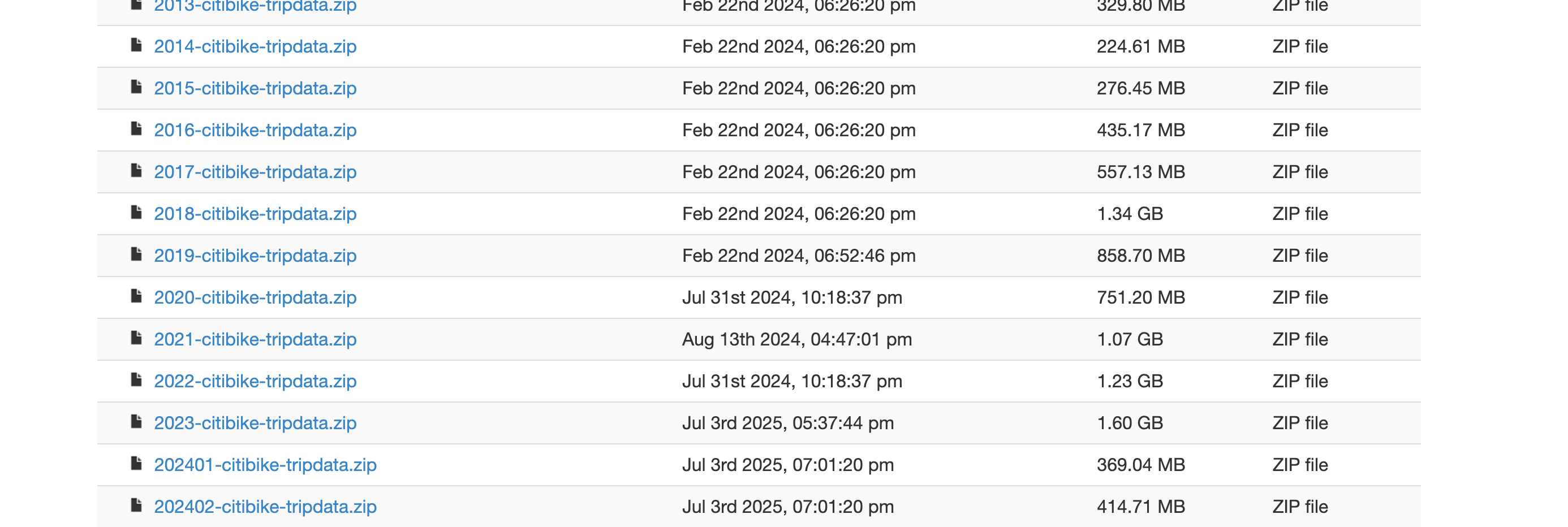
Step 2: Download Jersey Data
The file index contains many .zip files.
Each file usually represents one month.
# eval: true
from pathlib import Path
from urllib.request import urlretrieve
from zipfile import ZipFile

file_name = f"JC-{PERIOD}-citibike-tripdata.zip"

output_dir = Path(OUTPUT_DIR)
output_dir.mkdir(exist_ok=True)

zip_path = output_dir / file_name


## Dowloading the Zip file
url = f"{CITIBIKE_INDEX_URL}/{file_name}"

print(f"Downloading: {url}")
urlretrieve(url, zip_path)

print(f"Saved ZIP file to: {zip_path}")


with ZipFile(zip_path, "r") as zip_ref:
    zip_ref.extractall(output_dir)

print(f"Extracted files into: {output_dir}")
Downloading: https://s3.amazonaws.com/tripdata/JC-202510-citibike-tripdata.zip
Saved ZIP file to: ../../lab/python/data/citibike/JC-202510-citibike-tripdata.zip
Extracted files into: ../../lab/python/data/citibike
Importantremove the zip file
Once we get it we can remove the zip file
zip_path.unlink()
print("ZIP file removed.")
ZIP file removed.Step 3: Read the Data
Once we downloaded and effectively extracted the zip file, now we can read the data
file_name  = 'JC-202510-citibike-tripdata.csv'
citibike_202510 = pd.reada_csv(f'{output_dir}/{file_name}')
citibike_202510.head()| ride_id | rideable_type | started_at | ended_at | start_station_name | start_station_id | end_station_name | end_station_id | start_lat | start_lng | end_lat | end_lng | member_casual | |
|---|---|---|---|---|---|---|---|---|---|---|---|---|---|
| 0 | 929852F0DC04F49C | electric_bike | 2025-10-08 06:59:53.767 | 2025-10-08 07:04:08.012 | Warren St | JC006 | Essex Light Rail | NaN | 40.721124 | -74.038051 | NaN | NaN | member |
| 1 | 7E6F8FADF45B1D8E | electric_bike | 2025-10-08 08:13:15.096 | 2025-10-08 08:18:16.168 | Newark Ave | JC032 | Essex Light Rail | NaN | 40.721525 | -74.046305 | NaN | NaN | member |
| 2 | 9B679869FCA8F845 | electric_bike | 2025-10-09 10:10:26.020 | 2025-10-09 10:20:08.505 | Liberty Light Rail | JC052 | Newport PATH | NaN | 40.711242 | -74.055701 | NaN | NaN | member |
| 3 | E2051DD457BC4076 | electric_bike | 2025-10-09 11:34:22.937 | 2025-10-09 11:48:49.501 | Hoboken Ave at Monmouth St | JC105 | Newport PATH | NaN | 40.735208 | -74.046964 | NaN | NaN | member |
| 4 | 239AC07371E414EC | electric_bike | 2025-10-23 19:24:16.237 | 2025-10-23 19:28:22.592 | Union St & Bergen Ave | JC122 | Garfield Light Rail | JC119 | 40.715750 | -74.078870 | 40.710526 | -74.070112 | member |
Step 4: Downloading year 2025
Here we need one function which will help as to create an iterator
def period_iterator(year:list,start_m:int, stop_m:int)->list:
    """

    """
    YEAR = year
    MONTH =  [str(i+1) if i+1>9 else "0" + str(i+1) for i in range(start_m, stop_m)]

    periods = []

    for i in YEAR:
        for j in MONTH:
            k = i+j
            periods.append(k)
    # print(periods)
    return periods
periods = period_iterator(year = ['2025'],start_m = 1, stop_m = 12)
periods['202502',
'202503',
'202504',
'202505',
'202506',
'202507',
'202508',
'202509',
'202510',
'202511',
'202512']Once we have the iterator, we can now go over the loop and try to:
- donload each period
- extract
- remove the zip file
from pathlib import Path
from urllib.request import urlretrieve
from zipfile import ZipFile
from urllib.request import urlretrieve
from urllib.error import HTTPError, URLError

CITIBIKE_INDEX_URL = "https://s3.amazonaws.com/tripdata"
OUTPUT_DIR = "../data/citibike"
output_dir = Path(OUTPUT_DIR)
output_dir.mkdir(exist_ok=True)


for i in PERIODS:

    try:
        file_name = f"JC-{i}-citibike-tripdata.csv.zip"
        url = f"{CITIBIKE_INDEX_URL}/{file_name}"

        zip_path = output_dir / file_name
        urlretrieve(url, zip_path)

    except (HTTPError, URLError, FileNotFoundError):
        file_name = f"JC-{i}-citibike-tripdata.zip"
        url = f"{CITIBIKE_INDEX_URL}/{file_name}"

        zip_path = output_dir / file_name
        urlretrieve(url, zip_path)

    with ZipFile(zip_path, "r") as zip_ref:
        zip_ref.extractall(output_dir)
    print(f'{file_name}  Extracted')
    zip_path.unlink()
    print(f"{file_name} removed.")
Important
There might be inconsistant labeling in one or two files, think about how can we handle them!
Step 5: Removing __MACOSX
Once we downloaded and extracted the files, we can remove the __MACOSX folder if it exists.
In order to remove the __MACOSX folder we can use shutil package and rmtree() function
import shutil

shutil.rmtree(output_dir / "__MACOSX")
Note
__MACOSX file is a cache file which is created by the MAC operating system, it is not needed for our analysis, so we can remove it.
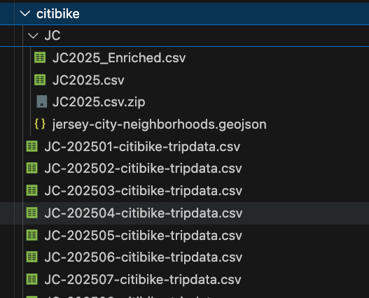
Step 6: Concatinating
Once we have all the csv files we can appending:
- we need to check all the filenames which are in the
../data/citibike/*.csv - read those csv files
- store it the list object named
dfs - use
pd.concat()to append them
import glob
import numpy as np
import pandas as pd

file_names = glob.glob(f'{output_dir}/*.csv')


dfs = []
cols = []
for file_name in file_names:
    df = pd.read_csv(file_name)
    print(df.columns, 2*"||",len(df.columns))

    cols.append(list(df.columns))
    dfs.append(df)
Index(['ride_id', 'rideable_type', 'started_at', 'ended_at',
'start_station_name', 'start_station_id', 'end_station_name',
'end_station_id', 'start_lat', 'start_lng', 'end_lat', 'end_lng',
'member_casual'],
dtype='str') |||| 13
Index(['ride_id', 'rideable_type', 'started_at', 'ended_at',
'start_station_name', 'start_station_id', 'end_station_name',
'end_station_id', 'start_lat', 'start_lng', 'end_lat', 'end_lng',
'member_casual'],
dtype='str') |||| 13
Index(['ride_id', 'rideable_type', 'started_at', 'ended_at',
'start_station_name', 'start_station_id', 'end_station_name',
'end_station_id', 'start_lat', 'start_lng', 'end_lat', 'end_lng',
'member_casual'],
dtype='str') |||| 13
Index(['ride_id', 'rideable_type', 'started_at', 'ended_at',
'start_station_name', 'start_station_id', 'end_station_name',
'end_station_id', 'start_lat', 'start_lng', 'end_lat', 'end_lng',
'member_casual'],
dtype='str') |||| 13
Index(['ride_id', 'rideable_type', 'started_at', 'ended_at',
'start_station_name', 'start_station_id', 'end_station_name',
'end_station_id', 'start_lat', 'start_lng', 'end_lat', 'end_lng',
'member_casual'],
dtype='str') |||| 13
Index(['ride_id', 'rideable_type', 'started_at', 'ended_at',
'start_station_name', 'start_station_id', 'end_station_name',
'end_station_id', 'start_lat', 'start_lng', 'end_lat', 'end_lng',
'member_casual'],
dtype='str') |||| 13
Index(['ride_id', 'rideable_type', 'started_at', 'ended_at',
'start_station_name', 'start_station_id', 'end_station_name',
'end_station_id', 'start_lat', 'start_lng', 'end_lat', 'end_lng',
'member_casual'],
dtype='str') |||| 13
Index(['ride_id', 'rideable_type', 'started_at', 'ended_at',
'start_station_name', 'start_station_id', 'end_station_name',
'end_station_id', 'start_lat', 'start_lng', 'end_lat', 'end_lng',
'member_casual'],
dtype='str') |||| 13
Index(['ride_id', 'rideable_type', 'started_at', 'ended_at',
'start_station_name', 'start_station_id', 'end_station_name',
'end_station_id', 'start_lat', 'start_lng', 'end_lat', 'end_lng',
'member_casual'],
dtype='str') |||| 13
Index(['ride_id', 'rideable_type', 'started_at', 'ended_at',
'start_station_name', 'start_station_id', 'end_station_name',
'end_station_id', 'start_lat', 'start_lng', 'end_lat', 'end_lng',
'member_casual'],
dtype='str') |||| 13
Index(['ride_id', 'rideable_type', 'started_at', 'ended_at',
'start_station_name', 'start_station_id', 'end_station_name',
'end_station_id', 'start_lat', 'start_lng', 'end_lat', 'end_lng',
'member_casual'],
dtype='str') |||| 13
Index(['ride_id', 'rideable_type', 'started_at', 'ended_at',
'start_station_name', 'start_station_id', 'end_station_name',
'end_station_id', 'start_lat', 'start_lng', 'end_lat', 'end_lng',
'member_casual'],
dtype='str') |||| 13citibike_df = pd.concat(dfs)
citibike_df.head()| ride_id | rideable_type | started_at | ended_at | start_station_name | start_station_id | end_station_name | end_station_id | start_lat | start_lng | end_lat | end_lng | member_casual | |
|---|---|---|---|---|---|---|---|---|---|---|---|---|---|
| 0 | 04CF7A399050E404 | classic_bike | 2025-02-22 17:40:16.500 | 2025-02-22 17:47:22.479 | Jersey & 3rd | JC074 | Van Vorst Park | JC035 | 40.723332 | -74.045953 | 40.718489 | -74.047727 | casual |
| 1 | 124AC7493E82D845 | classic_bike | 2025-02-21 12:28:13.319 | 2025-02-21 12:35:44.762 | Jersey & 3rd | JC074 | Columbus Drive | JC014 | 40.723332 | -74.045953 | 40.718355 | -74.038914 | member |
| 2 | 1A3BCA838E968327 | classic_bike | 2025-02-01 14:17:43.272 | 2025-02-01 14:59:09.894 | Jersey & 3rd | JC074 | Grove St PATH | JC115 | 40.723332 | -74.045953 | 40.719410 | -74.043090 | casual |
| 3 | 5994017EE989D6EE | electric_bike | 2025-02-22 11:36:29.292 | 2025-02-22 11:49:51.531 | Jersey & 3rd | JC074 | Jersey & 3rd | JC074 | 40.723332 | -74.045953 | 40.723332 | -74.045953 | casual |
| 4 | F81BCB97915C6BE6 | electric_bike | 2025-02-28 22:56:26.546 | 2025-02-28 23:07:40.391 | Jersey & 3rd | JC074 | Monroe St & 11 St | HB508 | 40.723332 | -74.045953 | 40.750109 | -74.036637 | casual |
Important
Once we have concatinated the yearly data, we can also save it properly in the respective folder.
We need this in order not to rerun the steps
citibike_df.to_csv("../data/citibike/JC2025.csv", index = False)Step 7: Setting Dates
citibike_df['started_at'] = pd.to_datetime(citibike_df['started_at'],errors="coerce")
citibike_df['ended_at'] = pd.to_datetime(citibike_df['ended_at'],errors="coerce")
Step 8: df overview
The available columns are:
citibike_df.columnsIndex(['ride_id', 'rideable_type', 'started_at', 'ended_at',
'start_station_name', 'start_station_id', 'end_station_name',
'end_station_id', 'start_lat', 'start_lng', 'end_lat', 'end_lng',
'member_casual'],
dtype='str')The dataset contains three important groups of variables:
| Variable Group | Columns | Meaning |
|---|---|---|
| Trip identifiers | ride_id, rideable_type, member_casual |
ride ID, bike type, and user type |
| Time variables | started_at, ended_at |
when the ride started and ended |
| Start location | start_station_name, start_station_id, start_lat, start_lng |
where the ride started |
| End location | end_station_name, end_station_id, end_lat, end_lng |
where the ride ended |
Step 9: Missing Values
missing_values = (
    citibike_df
    .isna()
    .sum()
    .reset_index()
)

missing_values.columns = ["column", "missing_count"]

missing_values["missing_share"] = (
    missing_values["missing_count"] / len(citibike_df)
)

missing_values.sort_values("missing_count", ascending=False)| column | missing_count | missing_share | |
|---|---|---|---|
| 7 | end_station_id | 4397 | 0.004385 |
| 10 | end_lat | 3444 | 0.003435 |
| 11 | end_lng | 3444 | 0.003435 |
| 6 | end_station_name | 3235 | 0.003226 |
| 4 | start_station_name | 3 | 0.000003 |
| 5 | start_station_id | 3 | 0.000003 |
| 8 | start_lat | 2 | 0.000002 |
| 9 | start_lng | 2 | 0.000002 |
| 0 | ride_id | 0 | 0.000000 |
| 3 | ended_at | 0 | 0.000000 |
| 2 | started_at | 0 | 0.000000 |
| 1 | rideable_type | 0 | 0.000000 |
| 12 | member_casual | 0 | 0.000000 |
Step 10: Ride Duration
Now we create ride duration.
citibike_df["ride_duration_minutes"] = (
    citibike_df["ended_at"] - citibike_df["started_at"]
).dt.total_seconds() / 60
We remove records with missing time values or invalid ride duration.
Important
Since, our goal is geographical analysis, we must drop the missing values or invalid ride durations
citibike_df = citibike_df.dropna(
    subset=[
        "ride_id",
        "started_at",
        "ended_at",
        "start_lat",
        "start_lng",
        "end_lat",
        "end_lng"
    ]
)

citibike_df = citibike_df[
    (citibike_df["ride_duration_minutes"] > 1) &
    (citibike_df["ride_duration_minutes"] <= 24 * 60)
].copy()
Important
- The lower bound removes extremely short trips.
- The upper bound removes trips longer than one day.
These values may represent docking issues, testing behavior, or unusual cases.
Step 11: Time Based Variables
For later aggregation, we create useful time columns.
citibike_df["date"] = citibike_df["started_at"].dt.date
citibike_df["month"] = citibike_df["started_at"].dt.to_period("M").astype(str)
citibike_df["month_name"] = citibike_df["started_at"].dt.month_name()
citibike_df["day_of_week"] = citibike_df["started_at"].dt.day_name()
citibike_df["hour"] = citibike_df["started_at"].dt.hour
def assign_season(month_number):
if month_number in [12, 1, 2]:
return "Winter"
elif month_number in [3, 4, 5]:
return "Spring"
elif month_number in [6, 7, 8]:
return "Summer"
else:
return "Autumn"
citibike_df["season"] = (
citibike_df["started_at"]
.dt.month
.apply(assign_season)
)citibike_df[
[
"started_at",
"date",
"month",
"month_name",
"day_of_week",
"hour",
"season"
]
].head()| started_at | date | month | month_name | day_of_week | hour | season | |
|---|---|---|---|---|---|---|---|
| 0 | 2025-02-22 17:40:16.500 | 2025-02-22 | 2025-02 | February | Saturday | 17 | Winter |
| 1 | 2025-02-21 12:28:13.319 | 2025-02-21 | 2025-02 | February | Friday | 12 | Winter |
| 2 | 2025-02-01 14:17:43.272 | 2025-02-01 | 2025-02 | February | Saturday | 14 | Winter |
| 3 | 2025-02-22 11:36:29.292 | 2025-02-22 | 2025-02 | February | Saturday | 11 | Winter |
| 4 | 2025-02-28 22:56:26.546 | 2025-02-28 | 2025-02 | February | Friday | 22 | Winter |
Once we have created all the required derived columns we can save the data again as JC2025_Enriched.csv file
citibike_df.to_csv("../data/citibike/JC/JC2025_Enriched.csv", index = False)
Important
Pay attention to location you must save the data in seperate folder in order to avoid problems during the re-run
Step 12: Getting Weather Data
USA government provides an API to download and analyze the weather data
import pandas as pd
import requests

lat = 40.7178
lng = -74.0431

start_date = "2025-01-01"
end_date = "2025-12-31"

url = "https://archive-api.open-meteo.com/v1/archive"

params = {
    "latitude": lat,
    "longitude": lng,
    "start_date": start_date,
    "end_date": end_date,
    "daily": [
        "temperature_2m_max",
        "temperature_2m_min",
        "temperature_2m_mean",
        "precipitation_sum",
        "rain_sum",
        "snowfall_sum",
        "wind_speed_10m_max"
    ],
    "timezone": "America/New_York"
}

response = requests.get(url, params=params)
response.raise_for_status()

data = response.json()

weather_daily = pd.DataFrame(data["daily"])
weather_daily["date"] = pd.to_datetime(weather_daily["time"])
weather_daily = weather_daily.drop(columns="time")

weather_daily.head()
Important
Again, likewise with the citibike data we can try to save it:
weather_daily.to_csv('../data/citibike/JC/jersey_weather_2025.csv', index = False)Weather Time Series Visualization
Now that we have selected the main daily weather columns, we can create simple time series visualizations.
We will focus on two variables:
- daily average temperature
- maximum daily wind speed
Before creating a time series plot, the date column should be in datetime format.
weather_daily["date"] = pd.to_datetime(weather_daily["date"])

weather_daily.dtypes
date datetime64[us]
temperature_2m_max float64
temperature_2m_min float64
temperature_2m_mean float64
precipitation_sum float64
rain_sum float64
snowfall_sum float64
wind_speed_10m_max float64
dtype: object
Important
As you can see the date column type is datetime64[us].
Daily Average Temperature Time Series
The column temperature_2m_mean represents the daily average temperature.
A line chart is useful here because we want to see how temperature changes over time.
fig = px.line(
    weather_daily,
    x="date",
    y="temperature_2m_mean",
    title="Daily Average Temperature Over Time",
    markers=False
)

fig.update_layout(
    xaxis_title="Date",
    yaxis_title="Average Temperature",
    hovermode="x unified"
)

fig.show()
This chart helps us see the seasonal pattern of temperature.
Usually, we expect lower temperatures in winter and higher temperatures in summer and the above chart shows exaclty that!
Important
Here we can use different appraches doing the way as we used to do previously: adding lines one by line, however we can make this even more efficient by converting the dataframe from wind format into long format
flowchart LR

    A["Wide Format<br><br>One row per date<br>Each measurement has its own column"] --> B["pd.melt()"]

    B --> C["Long Format<br><br>One row per date-variable pair<br>Variable names become values"]

    A1["date"] --> A
    A2["temperature_2m_max"] --> A
    A3["temperature_2m_min"] --> A
    A4["temperature_2m_mean"] --> A

    C --> C1["date"]
    C --> C2["temperature_type"]
    C --> C3["temperature"]
Daily Min/Max/Mean Tempreture
temperature_long = weather_daily.melt(
    id_vars="date",
    value_vars=[
        "temperature_2m_max",
        "temperature_2m_min",
        "temperature_2m_mean"
    ],
    var_name="temperature_type",
    value_name="temperature"
)

temperature_long.head()| date | temperature_type | temperature | |
|---|---|---|---|
| 0 | 2025-01-01 | temperature_2m_max | 10.9 |
| 1 | 2025-01-02 | temperature_2m_max | 5.4 |
| 2 | 2025-01-03 | temperature_2m_max | 3.2 |
| 3 | 2025-01-04 | temperature_2m_max | -0.1 |
| 4 | 2025-01-05 | temperature_2m_max | 0.3 |
fig = px.line(
    temperature_long,
    x="date",
    y="temperature",
    color="temperature_type",
    title="Daily Temperature: Maximum, Minimum, and Average",
    markers=False
)

fig.update_layout(
    xaxis_title="Date",
    yaxis_title="Temperature",
    hovermode="x unified"
)

fig.show()
This chart shows the daily temperature range.
The gap between maximum and minimum temperature shows how much temperature changes within a day.
Tip
hovermode="x unified" means to show all the values for each line.
Daily Wind Speed Time Series
The column wind_speed_10m_max represents the maximum daily wind speed.
This chart helps us identify windy periods.
Later, we can check whether high wind speed is associated with lower Citi Bike usage.
Step 13: Homework
- Create
Line Chartnumber of rides per months - Create
bar-plotnumber of rides per season - Bar Plot top 10 stations:
- start station
- end station
- Merge with the weather data to see some patterns
- Create Points
- Top Lines
Step 14: Homework Solution
Number of rides per monhts
First, we create a monthly aggregation.
Each row will represent one month.
monthly_rides = (
    citibike_df
    .groupby("month", as_index=False)
    .agg(
        number_of_rides=("ride_id", "count")
    )
)

monthly_rides| month | number_of_rides | |
|---|---|---|
| 0 | 2024-12 | 2 |
| 1 | 2025-01 | 50589 |
| 2 | 2025-02 | 45250 |
| 3 | 2025-03 | 73277 |
| 4 | 2025-04 | 81533 |
| 5 | 2025-05 | 93202 |
| 6 | 2025-06 | 96736 |
| 7 | 2025-07 | 107374 |
| 8 | 2025-08 | 108001 |
| 9 | 2025-09 | 115580 |
| 10 | 2025-10 | 103586 |
| 11 | 2025-11 | 76233 |
| 12 | 2025-12 | 47862 |
Now let’s try to visualize visualize the number of rides per month.
fig = px.bar(
    monthly_rides,
    x="month",
    y="number_of_rides",
    title="Number of Citi Bike Rides per Month"
)

fig.update_layout(
    xaxis_title="Month",
    yaxis_title="Number of Rides",
)

fig.show()
Tip
Try to highlight the top month
Number of Rides per Season
Now we aggregate the data by season.
season_rides = (
    citibike_df
    .groupby("season", as_index=False)
    .agg(
        number_of_rides=("ride_id", "count")
    )
)

season_order = ["Winter", "Spring", "Summer", "Autumn"]

season_rides["season"] = pd.Categorical(
    season_rides["season"],
    categories=season_order,
    ordered=True
)

season_rides = season_rides.sort_values("season")

season_rides| season | number_of_rides | |
|---|---|---|
| 3 | Winter | 143703 |
| 1 | Spring | 248012 |
| 2 | Summer | 312111 |
| 0 | Autumn | 295399 |
fig = px.bar(
    season_rides,
    x="season",
    y="number_of_rides",
    title="Number of Citi Bike Rides per Season",
    text_auto=True
)

fig.update_layout(
    xaxis_title="Season",
    yaxis_title="Number of Rides"
)

fig.show()
This chart compares total ride activity across seasons.
Usually, warmer seasons are expected to have more rides, while winter may have fewer rides due to colder weather, snow, wind, and shorter daylight hours.
Top 10 Start Stations
First, we calculate the top 10 stations by number of departures.
top_start_stations = (
    citibike_df
    .dropna(subset=["start_station_name"])
    .groupby("start_station_name", as_index=False)
    .agg(
        number_of_departures=("ride_id", "count")
    )
    .sort_values("number_of_departures", ascending=False)
    .head(10)
)

top_start_stations| start_station_name | number_of_departures | |
|---|---|---|
| 52 | Grove St PATH | 45004 |
| 58 | Hoboken Terminal - Hudson St & Hudson Pl | 25889 |
| 53 | Hamilton Park | 22259 |
| 95 | River St & Newark St | 21383 |
| 86 | Newport PATH | 20663 |
| 18 | Bergen Ave & Sip Ave | 20398 |
| 44 | Exchange Pl | 20008 |
| 0 | 11 St & Washington St | 19481 |
| 94 | River St & 1 St | 19143 |
| 87 | Newport Pkwy | 18720 |
fig = px.bar(
    top_start_stations.sort_values("number_of_departures"),
    x="number_of_departures",
    y="start_station_name",
    orientation="h",
    title="Top 10 Start Stations by Number of Departures",
    text_auto=True
)

fig.update_layout(
    xaxis_title="Number of Departures",
    yaxis_title="Start Station"
)

fig.show()
Interpretation
These stations are the most common origins of Citi Bike rides.
High departure volume may indicate stations near residential areas, transit hubs, offices, universities, or busy public locations.
REMEMBER to check them during the next session.
Top 10 End Stations
Now we calculate the top 10 stations by number of arrivals.
top_end_stations = (
    citibike_df
    .dropna(subset=["end_station_name"])
    .groupby("end_station_name", as_index=False)
    .agg(
        number_of_arrivals=("ride_id", "count")
    )
    .sort_values("number_of_arrivals", ascending=False)
    .head(10)
)

top_end_stations| end_station_name | number_of_arrivals | |
|---|---|---|
| 232 | Grove St PATH | 47758 |
| 241 | Hoboken Terminal - Hudson St & Hudson Pl | 26639 |
| 233 | Hamilton Park | 22353 |
| 347 | River St & Newark St | 22113 |
| 317 | Newport PATH | 20701 |
| 73 | Bergen Ave & Sip Ave | 20368 |
| 207 | Exchange Pl | 20160 |
| 7 | 11 St & Washington St | 19505 |
| 318 | Newport Pkwy | 18707 |
| 346 | River St & 1 St | 18515 |
fig = px.bar(
    top_end_stations.sort_values("number_of_arrivals"),
    x="number_of_arrivals",
    y="end_station_name",
    orientation="h",
    title="Top 10 End Stations by Number of Arrivals",
    text_auto=True
)

fig.update_layout(
    xaxis_title="Number of Arrivals",
    yaxis_title="End Station"
)

fig.show()
Interpretation
These stations are the most common destinations of Citi Bike rides.
High arrival volume may indicate stations near workplaces, shopping areas, public transportation, parks, or popular city destinations.
Merge with Weather Data to See Patterns
daily_rides = (
    citibike_df
    .groupby("date", as_index=False)
    .agg(
        number_of_rides=("ride_id", "count")
    )
)
daily_rides["date"] = pd.to_datetime(daily_rides["date"])
daily_rides.head()| date | number_of_rides | |
|---|---|---|
| 0 | 2024-12-31 | 2 |
| 1 | 2025-01-01 | 1179 |
| 2 | 2025-01-02 | 1710 |
| 3 | 2025-01-03 | 1770 |
| 4 | 2025-01-04 | 1337 |
Now let’s recall we prepare the weather date column.
weather_daily.head()| date | temperature_2m_max | temperature_2m_min | temperature_2m_mean | precipitation_sum | rain_sum | snowfall_sum | wind_speed_10m_max | |
|---|---|---|---|---|---|---|---|---|
| 0 | 2025-01-01 | 10.9 | 3.9 | 7.4 | 4.5 | 4.5 | 0.0 | 23.2 |
| 1 | 2025-01-02 | 5.4 | 0.3 | 2.6 | 0.0 | 0.0 | 0.0 | 25.1 |
| 2 | 2025-01-03 | 3.2 | -1.9 | 0.4 | 0.0 | 0.0 | 0.0 | 17.1 |
| 3 | 2025-01-04 | -0.1 | -2.7 | -1.4 | 0.0 | 0.0 | 0.0 | 26.1 |
| 4 | 2025-01-05 | 0.3 | -3.6 | -2.2 | 0.0 | 0.0 | 0.0 | 19.9 |
Now we merge the two datasets.
bike_weather_daily = daily_rides.merge(
    weather_daily,
    on="date",
    how="left"
)

bike_weather_daily.head()| date | number_of_rides | temperature_2m_max | temperature_2m_min | temperature_2m_mean | precipitation_sum | rain_sum | snowfall_sum | wind_speed_10m_max | |
|---|---|---|---|---|---|---|---|---|---|
| 0 | 2024-12-31 | 2 | NaN | NaN | NaN | NaN | NaN | NaN | NaN |
| 1 | 2025-01-01 | 1179 | 10.9 | 3.9 | 7.4 | 4.5 | 4.5 | 0.0 | 23.2 |
| 2 | 2025-01-02 | 1710 | 5.4 | 0.3 | 2.6 | 0.0 | 0.0 | 0.0 | 25.1 |
| 3 | 2025-01-03 | 1770 | 3.2 | -1.9 | 0.4 | 0.0 | 0.0 | 0.0 | 17.1 |
| 4 | 2025-01-04 | 1337 | -0.1 | -2.7 | -1.4 | 0.0 | 0.0 | 0.0 | 26.1 |
Check missing values after the merge.
bike_weather_daily.isna().sum()date 0
number_of_rides 0
temperature_2m_max 1
temperature_2m_min 1
temperature_2m_mean 1
precipitation_sum 1
rain_sum 1
snowfall_sum 1
wind_speed_10m_max 1
dtype: int64Rides and Average Temperature
fig = px.scatter(
    bike_weather_daily,
    x="temperature_2m_mean",
    y="number_of_rides",
    trendline="ols",
    title="Daily Rides vs Average Temperature"
)

fig.update_layout(
    xaxis_title="Average Daily Temperature",
    yaxis_title="Number of Rides"
)

fig.show()
Rides and Wind Speed
fig = px.scatter(
    bike_weather_daily,
    x="wind_speed_10m_max",
    y="number_of_rides",
    trendline="ols",
    title="Daily Rides vs Maximum Wind Speed"
)

fig.update_layout(
    xaxis_title="Maximum Wind Speed",
    yaxis_title="Number of Rides"
)

fig.show()
Rides and Precipitation
fig = px.scatter(
    bike_weather_daily,
    x="precipitation_sum",
    y="number_of_rides",
    trendline="ols",
    title="Daily Rides vs Precipitation"
)

fig.update_layout(
    xaxis_title="Daily Precipitation",
    yaxis_title="Number of Rides"
)

fig.show()
Dual y axis | rides vs temperature
Here we need to use more complex graph using plotly’s graph objects
import plotly.graph_objects as go


fig = go.Figure()

fig.add_trace(
    go.Scatter(
        x=bike_weather_daily["date"],
        y=bike_weather_daily["number_of_rides"],
        mode="lines",
        name="Daily Rides",
        yaxis="y1"
    )
)

fig.add_trace(
    go.Scatter(
        x=bike_weather_daily["date"],
        y=bike_weather_daily["temperature_2m_mean"],
        mode="lines",
        name="Daily Average Temperature",
        yaxis="y2"
    )
)

fig.update_layout(
    title="Daily Rides and Daily Average Temperature",
    xaxis=dict(
        title="Day"
    ),
    yaxis=dict(
        title="Daily Rides",
        side="left"
    ),
    yaxis2=dict(
        title="Daily Average Temperature",
        overlaying="y",
        side="right"
    ),
    hovermode="x unified",
    legend=dict(
        orientation="h",
        yanchor="bottom",
        y=1.02,
        xanchor="right",
        x=1
    )
)

fig.show()
Step 15: Geopandas
import geopandas as gpd
from urllib.parse import urlencode
from pathlib import Path


url = '../data/citibike/JC/jersey-city-neighborhoods.geojson'

jersey_city = gpd.read_file(url)

jersey_city.head()| cartodb_id | area_sq_ft | acres | area | neighborhood | color | lon | lat | geometry | |
|---|---|---|---|---|---|---|---|---|---|
| 0 | 38 | 411601381.8 | 9449.068 | Greenville | Port Liberte | NaN | -74.074540 | 40.694202 | POLYGON ((-74.06862 40.70098, -74.06808 40.696... |
| 1 | 52 | 411601381.8 | 9449.068 | Bergen-Lafayette | LSP Industrial | NaN | -74.062358 | 40.699189 | POLYGON ((-74.06808 40.69684, -74.06862 40.700... |
| 2 | 29 | 411601381.8 | 9449.068 | West Side | Hackensack | NaN | -74.085147 | 40.735520 | POLYGON ((-74.07601 40.73822, -74.07781 40.737... |
| 3 | 35 | 411601381.8 | 9449.068 | Bergen-Lafayette | Lafayette | 12.0 | -74.061279 | 40.712676 | POLYGON ((-74.056 40.71735, -74.056 40.71692, ... |
| 4 | 51 | 411601381.8 | 9449.068 | Greenville | Jackson Hill | 15.0 | -74.085503 | 40.700791 | POLYGON ((-74.07561 40.70233, -74.0758 40.7020... |
After reading a spatial file, always check the basic structure.
jersey_city.info()<class 'geopandas.geodataframe.GeoDataFrame'>
RangeIndex: 53 entries, 0 to 52
Data columns (total 9 columns):
# Column Non-Null Count Dtype
--- ------ -------------- -----
0 cartodb_id 53 non-null int32
1 area_sq_ft 53 non-null float64
2 acres 53 non-null float64
3 area 53 non-null str
4 neighborhood 53 non-null str
5 color 18 non-null float64
6 lon 53 non-null float64
7 lat 53 non-null float64
8 geometry 53 non-null geometry
dtypes: float64(5), geometry(1), int32(1), str(2)
memory usage: 4.8 KBjersey_city.crs<Geographic 2D CRS: EPSG:4326>
Name: WGS 84
Axis Info [ellipsoidal]:
- Lat[north]: Geodetic latitude (degree)
- Lon[east]: Geodetic longitude (degree)
Area of Use:
- name: World.
- bounds: (-180.0, -90.0, 180.0, 90.0)
Datum: World Geodetic System 1984 ensemble
- Ellipsoid: WGS 84
- Prime Meridian: Greenwich
Important
Our geojson file has EPSG:4326 WGS 84.
This is good because EPSG:4326 is the standard latitude-longitude coordinate system used by:
- GPS coordinates
- GeoJSON files
- Folium maps
- most web mapping tools
jersey_city = jersey_city.to_crs("EPSG:4326")We can also plot the map by simply applying plot() method :)
jersey_city.plot()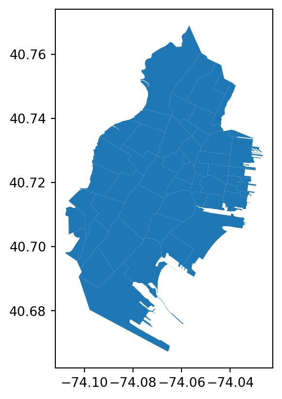
Citibike Points
in GeoPandas and Shapely, coordinates are stored as:
\[ (x, y) = (\text{longitude}, \text{latitude}) \]
So when creating points manually, the correct order is:
Station Level Summary
Now we create a station-level summary from citibike_df. The goal is to move from trip-level data to station-level data.
Each row in the final table will represent one station.
The final station summary will include:
| Column | Meaning |
|---|---|
station_id |
unique station identifier |
station_name |
station name |
lat |
station latitude |
lng |
station longitude |
total_departures |
number of rides starting from the station |
total_arrivals |
number of rides ending at the station |
total_activity |
departures plus arrivals |
net_departures |
departures minus arrivals |
In order to do so we need to create to dataframees and later merge them:
- departures: where each row in
station_departuresrepresents a station where rides started. - arrivals: where each row in
station_arrivalsrepresents a station where rides ended.
\[\downarrow\]
\[\text{merge departures and arrivals}\]
station_departures
start_stations = citibike_df[
    [
        "ride_id",
        "start_station_id",
        "start_station_name",
        "start_lat",
        "start_lng"
    ]
].copy()
Important
.copy() is used to create an independent dataframe from the selected columns.
Without .copy(), pandas may treat start_stations as a view of the original dataframe rather than a fully independent dataframe.
That can create warnings or unexpected behavior when we later modify it.
We use
.copy()to avoid accidental modification issues and to make surestart_stationsis a clean independent dataframe.
For example, after selecting the columns, we rename columns and add a new column as shown bellow.
start_stations = start_stations.rename(
    columns={
        "start_station_id": "station_id",
        "start_station_name": "station_name",
        "start_lat": "lat",
        "start_lng": "lng"
    }
)

start_stations["activity_type"] = "departure"
station_arrivals
end_stations = citibike_df[
    [
        "ride_id",
        "end_station_id",
        "end_station_name",
        "end_lat",
        "end_lng"
    ]
].copy()

end_stations = end_stations.rename(
    columns={
        "end_station_id": "station_id",
        "end_station_name": "station_name",
        "end_lat": "lat",
        "end_lng": "lng"
    }
)

end_stations["activity_type"] = "arrival"

end_stations.head()| ride_id | station_id | station_name | lat | lng | activity_type | |
|---|---|---|---|---|---|---|
| 0 | 04CF7A399050E404 | JC035 | Van Vorst Park | 40.718489 | -74.047727 | arrival |
| 1 | 124AC7493E82D845 | JC014 | Columbus Drive | 40.718355 | -74.038914 | arrival |
| 2 | 1A3BCA838E968327 | JC115 | Grove St PATH | 40.719410 | -74.043090 | arrival |
| 3 | 5994017EE989D6EE | JC074 | Jersey & 3rd | 40.723332 | -74.045953 | arrival |
| 4 | F81BCB97915C6BE6 | HB508 | Monroe St & 11 St | 40.750109 | -74.036637 | arrival |
Concatenate Departures and Arrivals
Now we combine both summaries.
This is similar to UNION ALL in SQL.
station_activity_long = pd.concat(
    [
        start_stations,
        end_stations
    ],
    ignore_index=True
)

station_activity_long = station_activity_long.dropna(
    subset=[
        "station_id",
        "station_name",
        "lat",
        "lng"
    ]
)

station_activity_long.head()| ride_id | station_id | station_name | lat | lng | activity_type | |
|---|---|---|---|---|---|---|
| 0 | 04CF7A399050E404 | JC074 | Jersey & 3rd | 40.723332 | -74.045953 | departure |
| 1 | 124AC7493E82D845 | JC074 | Jersey & 3rd | 40.723332 | -74.045953 | departure |
| 2 | 1A3BCA838E968327 | JC074 | Jersey & 3rd | 40.723332 | -74.045953 | departure |
| 3 | 5994017EE989D6EE | JC074 | Jersey & 3rd | 40.723332 | -74.045953 | departure |
| 4 | F81BCB97915C6BE6 | JC074 | Jersey & 3rd | 40.723332 | -74.045953 | departure |
Cleaning and Aggregating
At this point, the data is still not aggregated.
It has many rows per station.
station_activity_agg = (
    station_activity_long
    .groupby(
        [
            "station_id",
            "station_name",
            "lat",
            "lng",
            "activity_type"
        ],
        as_index=False
    )
    .agg(
        number_of_rides=("ride_id", "count")
    )
)

station_activity_agg.head()| station_id | station_name | lat | lng | activity_type | number_of_rides | |
|---|---|---|---|---|---|---|
| 0 | 3278.07 | Brooklyn Ave & Snyder Ave | 40.649150 | -73.943680 | arrival | 1 |
| 1 | 3344.02 | Park Circle & East Dr | 40.651566 | -73.972212 | arrival | 1 |
| 2 | 3480.04 | Parkside Ave & Flatbush Ave | 40.655630 | -73.959680 | arrival | 1 |
| 3 | 3579.04 | Windsor Pl & Howard Pl | 40.659491 | -73.980139 | arrival | 1 |
| 4 | 3762.08 | 10 St & 7 Ave | 40.666208 | -73.981999 | arrival | 1 |
Pivot the Data
Pivot to One Row per Station
Now we convert departure and arrival into separate columns.
station_summary = (
    station_activity_agg
    .pivot_table(
        index=[
            "station_id",
            "station_name",
            "lat",
            "lng"
        ],
        columns="activity_type",
        values="number_of_rides",
        fill_value=0
    )
    .reset_index()
)

station_summary.head()| activity_type | station_id | station_name | lat | lng | arrival | departure |
|---|---|---|---|---|---|---|
| 0 | 3278.07 | Brooklyn Ave & Snyder Ave | 40.649150 | -73.943680 | 1.0 | 0.0 |
| 1 | 3344.02 | Park Circle & East Dr | 40.651566 | -73.972212 | 1.0 | 0.0 |
| 2 | 3480.04 | Parkside Ave & Flatbush Ave | 40.655630 | -73.959680 | 1.0 | 0.0 |
| 3 | 3579.04 | Windsor Pl & Howard Pl | 40.659491 | -73.980139 | 1.0 | 0.0 |
| 4 | 3762.08 | 10 St & 7 Ave | 40.666208 | -73.981999 | 1.0 | 0.0 |
Rename and Create Final Metrics
station_summary = station_summary.rename(
    columns={
        "departure": "total_departures",
        "arrival": "total_arrivals"
    }
)

station_summary["total_activity"] = (
    station_summary["total_departures"] +
    station_summary["total_arrivals"]
)

station_summary["net_departures"] = (
    station_summary["total_departures"] -
    station_summary["total_arrivals"]
)

station_summary = station_summary.sort_values(
    "total_activity",
    ascending=False
).reset_index(drop=True)

station_summary.head()| activity_type | station_id | station_name | lat | lng | total_arrivals | total_departures | total_activity | net_departures |
|---|---|---|---|---|---|---|---|---|
| 0 | JC115 | Grove St PATH | 40.719410 | -74.043090 | 47744.0 | 45004.0 | 92748.0 | -2740.0 |
| 1 | HB101 | Hoboken Terminal - Hudson St & Hudson Pl | 40.735938 | -74.030305 | 26638.0 | 25889.0 | 52527.0 | -749.0 |
| 2 | JC009 | Hamilton Park | 40.727596 | -74.044247 | 22347.0 | 22259.0 | 44606.0 | -88.0 |
| 3 | HB106 | River St & Newark St | 40.736722 | -74.029007 | 22113.0 | 21383.0 | 43496.0 | -730.0 |
| 4 | JC066 | Newport PATH | 40.727224 | -74.033759 | 20698.0 | 20663.0 | 41361.0 | -35.0 |
gpd.points_from_xy(longitude, latitude)For Citi Bike stations, this means:
station_gdf = gpd.GeoDataFrame(
    station_summary,
    geometry=gpd.points_from_xy(
        station_summary["lng"],
        station_summary["lat"]
    ),
    crs="EPSG:4326"
)

station_gdf.head()| activity_type | station_id | station_name | lat | lng | total_arrivals | total_departures | total_activity | net_departures | geometry |
|---|---|---|---|---|---|---|---|---|---|
| 0 | JC115 | Grove St PATH | 40.719410 | -74.043090 | 47744.0 | 45004.0 | 92748.0 | -2740.0 | POINT (-74.04309 40.71941) |
| 1 | HB101 | Hoboken Terminal - Hudson St & Hudson Pl | 40.735938 | -74.030305 | 26638.0 | 25889.0 | 52527.0 | -749.0 | POINT (-74.0303 40.73594) |
| 2 | JC009 | Hamilton Park | 40.727596 | -74.044247 | 22347.0 | 22259.0 | 44606.0 | -88.0 | POINT (-74.04425 40.7276) |
| 3 | HB106 | River St & Newark St | 40.736722 | -74.029007 | 22113.0 | 21383.0 | 43496.0 | -730.0 | POINT (-74.02901 40.73672) |
| 4 | JC066 | Newport PATH | 40.727224 | -74.033759 | 20698.0 | 20663.0 | 41361.0 | -35.0 | POINT (-74.03376 40.72722) |
Step 16: Top Lines and Spatial Aggregation
At this point, we already have:
citibike_df: trip-level Citi Bike datajersey_city: Jersey City neighborhood polygonsstation_summary: station-level summary tablestation_gdf: station-level GeoDataFrame with point geometry
The previous section created station_gdf from station_summary by using longitude and latitude correctly. :contentReferenceoaicite:0
Now we will continue with two main directions:
- Draw top ride lines using
Folium - Conduct spatial joins to aggregate station activity by neighborhood and create choropleth maps
Why This Step Matters
So far, we have station-level points.
Now we want to connect those points to neighborhood polygons.
This allows us to move from:
\[ \text{Station-Level Analysis} \]
to:
\[ \text{Neighborhood-Level Analysis} \]
This is useful because dashboards and business reports usually need area-level insights, not only individual station-level details.
Creating Top Ride Lines
A ride line connects a start station to an end station.
In Citi Bike data, a route is defined as:
\[ \text{Start Station} \rightarrow \text{End Station} \]
Instead of plotting every individual ride, we aggregate rides by route.
This gives us one row per station-to-station connection.
Create Route-Level Summary
route_summary = (
    citibike_df
    .dropna(
        subset=[
            "start_station_id",
            "start_station_name",
            "end_station_id",
            "end_station_name",
            "start_lat",
            "start_lng",
            "end_lat",
            "end_lng"
        ]
    )
    .groupby(
        [
            "start_station_id",
            "start_station_name",
            "end_station_id",
            "end_station_name",
            "start_lat",
            "start_lng",
            "end_lat",
            "end_lng"
        ],
        as_index=False
    )
    .agg(
        number_of_rides=("ride_id", "count")
    )
    .sort_values("number_of_rides", ascending=False)
)

route_summary["route"] = (
    route_summary["start_station_name"] +
    " → " +
    route_summary["end_station_name"]
)

route_summary.head()| start_station_id | start_station_name | end_station_id | end_station_name | start_lat | start_lng | end_lat | end_lng | number_of_rides | route | |
|---|---|---|---|---|---|---|---|---|---|---|
| 83 | HB101 | Hoboken Terminal - Hudson St & Hudson Pl | JC105 | Hoboken Ave at Monmouth St | 40.735938 | -74.030305 | 40.735208 | -74.046964 | 4559 | Hoboken Terminal - Hudson St & Hudson Pl → Hob... |
| 5583 | JC055 | McGinley Square | JC109 | Bergen Ave & Sip Ave | 40.725340 | -74.067622 | 40.731009 | -74.064437 | 4306 | McGinley Square → Bergen Ave & Sip Ave |
| 8709 | JC115 | Grove St PATH | JC013 | Marin Light Rail | 40.719410 | -74.043090 | 40.714584 | -74.042817 | 4131 | Grove St PATH → Marin Light Rail |
| 3937 | JC013 | Marin Light Rail | JC115 | Grove St PATH | 40.714584 | -74.042817 | 40.719410 | -74.043090 | 3831 | Marin Light Rail → Grove St PATH |
| 8723 | JC115 | Grove St PATH | JC052 | Liberty Light Rail | 40.719410 | -74.043090 | 40.711242 | -74.055701 | 3750 | Grove St PATH → Liberty Light Rail |
Inspect Top Routes
top_routes = route_summary.head(20)

top_routes[
    [
        "route",
        "number_of_rides"
    ]
]| route | number_of_rides | |
|---|---|---|
| 83 | Hoboken Terminal - Hudson St & Hudson Pl → Hob... | 4559 |
| 5583 | McGinley Square → Bergen Ave & Sip Ave | 4306 |
| 8709 | Grove St PATH → Marin Light Rail | 4131 |
| 3937 | Marin Light Rail → Grove St PATH | 3831 |
| 8723 | Grove St PATH → Liberty Light Rail | 3750 |
| 8445 | Bergen Ave & Sip Ave → McGinley Square | 3609 |
| 5395 | Liberty Light Rail → Grove St PATH | 3605 |
| 8154 | Hoboken Ave at Monmouth St → Hoboken Terminal ... | 3257 |
| 4570 | Brunswick St → Grove St PATH | 3175 |
| 3788 | Hamilton Park → Grove St PATH | 2998 |
| 6228 | Morris Canal → Exchange Pl | 2753 |
| 16 | Hoboken Terminal - Hudson St & Hudson Pl → Sou... | 2726 |
| 7225 | Fairmount Ave → Bergen Ave & Sip Ave | 2613 |
| 8444 | Bergen Ave & Sip Ave → Lincoln Park | 2575 |
| 8708 | Grove St PATH → Hamilton Park | 2535 |
| 6745 | Lafayette Park → Grove St PATH | 2531 |
| 6559 | Dixon Mills → Grove St PATH | 2515 |
| 8755 | Grove St PATH → JC Medical Center | 2498 |
| 8737 | Grove St PATH → Lafayette Park | 2444 |
| 8715 | Grove St PATH → Brunswick St | 2343 |
Drawing Top Lines with Folium
We visualize only the top routes.
If we draw all routes, the map becomes too crowded.
import folium

top_lines = route_summary.head(100).copy()

center_lat = station_gdf["lat"].mean()
center_lng = station_gdf["lng"].mean()

line_map = folium.Map(
    location=[center_lat, center_lng],
    zoom_start=12
)

max_rides = top_lines["number_of_rides"].max()

for _, row in top_lines.iterrows():

    start_point = [
        row["start_lat"],
        row["start_lng"]
    ]

    end_point = [
        row["end_lat"],
        row["end_lng"]
    ]

    line_weight = 1 + (row["number_of_rides"] / max_rides) * 8

    folium.PolyLine(
        locations=[start_point, end_point],
        weight=line_weight,
        opacity=0.5,
        popup=f"""
        <b>{row['route']}</b><br>
        Number of Rides: {row['number_of_rides']}
        """
    ).add_to(line_map)

line_map
Make this Notebook Trusted to load map: File -> Trust Notebook
TipInterpretation
This map shows the most frequent station-to-station movements.
- thicker lines represent more rides
- shorter lines may represent local neighborhood movement
- longer lines may represent cross-neighborhood or cross-city trips
- dense line clusters may show important mobility corridors
This is more useful than plotting every ride because the map focuses on repeated patterns.
Spatial Join Between Stations and Neighborhoods
Now we connect station points with neighborhood polygons.
The spatial question is:
\[ \text{Which neighborhood contains each station?} \]
This is done using a spatial join.
Check CRS Before Spatial Join
Before a spatial join, both GeoDataFrames must have the same CRS.
Note
We have already checked above, however it is a recommended to check the projects everytime.
print("Station CRS:", station_gdf.crs)
print("Neighborhood CRS:", jersey_city.crs)
Station CRS: EPSG:4326
Neighborhood CRS: EPSG:4326Since both are already in EPSG:4326, we can keep them aligned.
station_gdf = station_gdf.to_crs("EPSG:4326")
jersey_city = jersey_city.to_crs("EPSG:4326")
Inspect Neighborhood Columns
Before joining and aggregating, we need to know which column contains the neighborhood name.
jersey_city.columnsIndex(['cartodb_id', 'area_sq_ft', 'acres', 'area', 'neighborhood', 'color',
'lon', 'lat', 'geometry'],
dtype='str')Spatial Join: Assign Stations to Neighborhoods
station_neighborhood = gpd.sjoin(
    station_gdf,
    jersey_city,
    how="inner",
    predicate="within"
)

station_neighborhood.head()| station_id | station_name | lat_left | lng | total_arrivals | total_departures | total_activity | net_departures | geometry | index_right | cartodb_id | area_sq_ft | acres | area | neighborhood | color | lon | lat_right | |
|---|---|---|---|---|---|---|---|---|---|---|---|---|---|---|---|---|---|---|
| 0 | JC115 | Grove St PATH | 40.719410 | -74.043090 | 47744.0 | 45004.0 | 92748.0 | -2740.0 | POINT (-74.04309 40.71941) | 49 | 2 | 411601381.8 | 9449.068 | Downtown | Van Vorst Park | 21.0 | -74.047234 | 40.718943 |
| 2 | JC009 | Hamilton Park | 40.727596 | -74.044247 | 22347.0 | 22259.0 | 44606.0 | -88.0 | POINT (-74.04425 40.7276) | 10 | 18 | 411601381.8 | 9449.068 | Downtown | Hamilton Park | 28.0 | -74.046672 | 40.727436 |
| 4 | JC066 | Newport PATH | 40.727224 | -74.033759 | 20698.0 | 20663.0 | 41361.0 | -35.0 | POINT (-74.03376 40.72722) | 8 | 12 | 411601381.8 | 9449.068 | Downtown | Newport | 22.0 | -74.034927 | 40.729255 |
| 5 | JC109 | Bergen Ave & Sip Ave | 40.731009 | -74.064437 | 20357.0 | 20398.0 | 40755.0 | 41.0 | POINT (-74.06444 40.73101) | 16 | 31 | 411601381.8 | 9449.068 | Journal Square | Journal Square | NaN | -74.063466 | 40.733757 |
| 6 | JC116 | Exchange Pl | 40.716366 | -74.034344 | 20142.0 | 20008.0 | 40150.0 | -134.0 | POINT (-74.03434 40.71637) | 48 | 13 | 411601381.8 | 9449.068 | Downtown | Exchange Place | 23.0 | -74.033539 | 40.716458 |
We use:
predicate="within"because we want stations that are located inside neighborhood polygons.
We use:
how="inner"because we want to keep only stations that are inside Jersey City neighborhood polygons.
This is important because some Citi Bike rides may connect to stations outside Jersey City.
Check How Many Stations Are Inside Jersey City
print("All stations:", len(station_gdf))
print("Stations inside Jersey City neighborhoods:", len(station_neighborhood))
All stations: 488
Stations inside Jersey City neighborhoods: 79If the number of stations decreases, that means some stations were outside the Jersey City neighborhood polygons.
That is expected if the dataset includes trips ending outside Jersey City.
Neighborhood-Level Summary
Now each station has neighborhood information.
We can aggregate station activity by neighborhood.
neighborhood_activity = (
    station_neighborhood
    .groupby('neighborhood', as_index=False)
    .agg(
        number_of_stations=("station_id", "nunique"),
        total_departures=("total_departures", "sum"),
        total_arrivals=("total_arrivals", "sum"),
        total_activity=("total_activity", "sum"),
        net_departures=("net_departures", "sum")
    )
)

neighborhood_activity["avg_activity_per_station"] = (
    neighborhood_activity["total_activity"] /
    neighborhood_activity["number_of_stations"]
)

neighborhood_activity = neighborhood_activity.sort_values(
    "total_activity",
    ascending=False
)

neighborhood_activity.head()| neighborhood | number_of_stations | total_departures | total_arrivals | total_activity | net_departures | avg_activity_per_station | |
|---|---|---|---|---|---|---|---|
| 25 | Van Vorst Park | 6 | 96210.0 | 98853.0 | 195063.0 | -2643.0 | 32510.500000 |
| 17 | Palus Hook | 6 | 59567.0 | 59160.0 | 118727.0 | 407.0 | 19787.833333 |
| 14 | Newport | 2 | 39383.0 | 39402.0 | 78785.0 | -19.0 | 39392.500000 |
| 10 | Journal Square | 3 | 33007.0 | 32560.0 | 65567.0 | 447.0 | 21855.666667 |
| 4 | Hamilton Park | 2 | 31762.0 | 31922.0 | 63684.0 | -160.0 | 31842.000000 |
Interpretation of Neighborhood Metrics
| Metric | Meaning |
|---|---|
number_of_stations |
number of Citi Bike stations in the neighborhood |
total_departures |
rides starting from stations in the neighborhood |
total_arrivals |
rides ending at stations in the neighborhood |
total_activity |
departures plus arrivals |
net_departures |
departures minus arrivals |
avg_activity_per_station |
average station usage intensity |
The metric total_activity is useful, but it can be misleading.
A neighborhood with many stations may naturally have more activity.
That is why we also calculate:
\[ \text{Average Activity per Station} = \frac{\text{Total Activity}}{\text{Number of Stations}} \]
Create Center Point for the Map
center_lat = station_gdf.geometry.y.mean()
center_lng = station_gdf.geometry.x.mean()

center_lat, center_lng
(np.float64(40.734012258630905), np.float64(-74.00137516113631))In GeoPandas point geometry:
\[ x = \text{longitude} \]
\[ y = \text{latitude} \]
So for Folium we use:
location=[row.geometry.y, row.geometry.x]because Folium expects:
[latitude, longitude]Visualize Each Station as a Point
station_point_map = folium.Map(
    location=[center_lat, center_lng],
    zoom_start=12
)

for _, row in station_gdf.iterrows():

    folium.CircleMarker(
        location=[
            row.geometry.y,
            row.geometry.x
        ],
        radius=5,
        popup=f"""
        <b>{row['station_name']}</b><br>
        Station ID: {row['station_id']}<br>
        Departures: {row['total_departures']:.0f}<br>
        Arrivals: {row['total_arrivals']:.0f}<br>
        Total Activity: {row['total_activity']:.0f}<br>
        Net Departures: {row['net_departures']:.0f}
        """,
        tooltip=row["station_name"],
        fill=True,
        fill_opacity=0.6,
        opacity=0.8
    ).add_to(station_point_map)

station_point_map
Make this Notebook Trusted to load map: File -> Trust Notebook
Merge Neighborhood Metrics Back to Polygons
To create a choropleth map, the metrics must be attached to the neighborhood polygons.
neighborhood_choropleth_gdf = jersey_city.merge(
    neighborhood_activity,
    on='neighborhood',
    how="left"
)

neighborhood_choropleth_gdf.head()| cartodb_id | area_sq_ft | acres | area | neighborhood | color | lon | lat | geometry | number_of_stations | total_departures | total_arrivals | total_activity | net_departures | avg_activity_per_station | |
|---|---|---|---|---|---|---|---|---|---|---|---|---|---|---|---|
| 0 | 38 | 411601381.8 | 9449.068 | Greenville | Port Liberte | NaN | -74.074540 | 40.694202 | POLYGON ((-74.06862 40.70098, -74.06808 40.696... | 1.0 | 12.0 | 9.0 | 21.0 | 3.0 | 21.000 |
| 1 | 52 | 411601381.8 | 9449.068 | Bergen-Lafayette | LSP Industrial | NaN | -74.062358 | 40.699189 | POLYGON ((-74.06808 40.69684, -74.06862 40.700... | NaN | NaN | NaN | NaN | NaN | NaN |
| 2 | 29 | 411601381.8 | 9449.068 | West Side | Hackensack | NaN | -74.085147 | 40.735520 | POLYGON ((-74.07601 40.73822, -74.07781 40.737... | NaN | NaN | NaN | NaN | NaN | NaN |
| 3 | 35 | 411601381.8 | 9449.068 | Bergen-Lafayette | Lafayette | 12.0 | -74.061279 | 40.712676 | POLYGON ((-74.056 40.71735, -74.056 40.71692, ... | 6.0 | 30896.0 | 30730.0 | 61626.0 | 166.0 | 10271.000 |
| 4 | 51 | 411601381.8 | 9449.068 | Greenville | Jackson Hill | 15.0 | -74.085503 | 40.700791 | POLYGON ((-74.07561 40.70233, -74.0758 40.7020... | 16.0 | 6173.0 | 6045.0 | 12218.0 | 128.0 | 763.625 |
Some neighborhoods may not have Citi Bike stations.
For those neighborhoods, the activity values will be missing.
We replace missing values with zero.
activity_columns = [
    "number_of_stations",
    "total_departures",
    "total_arrivals",
    "total_activity",
    "net_departures",
    "avg_activity_per_station"
]

neighborhood_choropleth_gdf[activity_columns] = (
    neighborhood_choropleth_gdf[activity_columns]
    .fillna(0)
)

neighborhood_choropleth_gdf[
    [
        'neighborhood',
        "number_of_stations",
        "total_departures",
        "total_arrivals",
        "total_activity",
        "avg_activity_per_station"
    ]
].head()| neighborhood | number_of_stations | total_departures | total_arrivals | total_activity | avg_activity_per_station | |
|---|---|---|---|---|---|---|
| 0 | Port Liberte | 1.0 | 12.0 | 9.0 | 21.0 | 21.000 |
| 1 | LSP Industrial | 0.0 | 0.0 | 0.0 | 0.0 | 0.000 |
| 2 | Hackensack | 0.0 | 0.0 | 0.0 | 0.0 | 0.000 |
| 3 | Lafayette | 6.0 | 30896.0 | 30730.0 | 61626.0 | 10271.000 |
| 4 | Jackson Hill | 16.0 | 6173.0 | 6045.0 | 12218.0 | 763.625 |
Step 17: Choropleth Map
Now we create a choropleth map.
We start with total_activity.
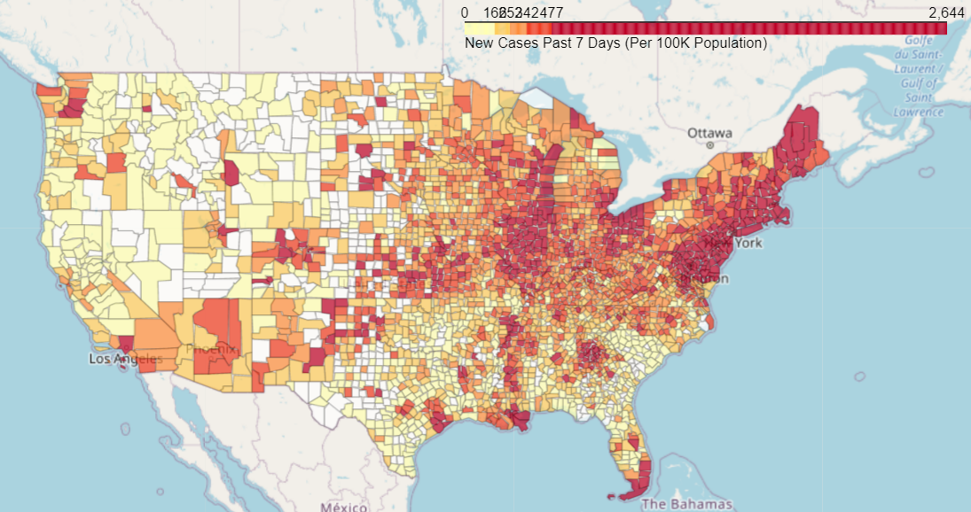
Helper Function for Folium Choropleth
To avoid repeating code, we create a small helper function.
def create_neighborhood_choropleth(
    gdf,
    metric,
    legend_name,
    neighborhood_col="neighborhood"
):
    choropleth_map = folium.Map(
        location=[center_lat, center_lng],
        zoom_start=12
    )

    folium.Choropleth(
        geo_data=gdf,
        data=gdf,
        columns=[neighborhood_col, metric],
        key_on=f"feature.properties.{neighborhood_col}",
        fill_opacity=0.7,
        line_opacity=0.4,
        legend_name=legend_name,
        nan_fill_opacity=0.1
    ).add_to(choropleth_map)

    folium.GeoJson(
        gdf,
        name="Neighborhood Boundaries",
        tooltip=folium.GeoJsonTooltip(
            fields=[
                neighborhood_col,
                metric
            ],
            aliases=[
                "Neighborhood:",
                f"{legend_name}:"
            ],
            localize=True
        ),
        style_function=lambda feature: {
            "fillOpacity": 0,
            "color": "black",
            "weight": 1
        }
    ).add_to(choropleth_map)

    folium.LayerControl().add_to(choropleth_map)

    return choropleth_map
Choropleth: Total Activity by Neighborhood
This choropleth shows which neighborhoods have the highest total Citi Bike station activity. However, neighborhoods with more stations may naturally appear more active. So this map should be interpreted together with the number of stations.
total_activity_map = create_neighborhood_choropleth(
    gdf=neighborhood_choropleth_gdf,
    metric="total_activity",
    legend_name="Total Citi Bike Activity",
    neighborhood_col="neighborhood"
)

total_activity_map
Make this Notebook Trusted to load map: File -> Trust Notebook
Choropleth by Number of Stations
station_count_map = create_neighborhood_choropleth(
    gdf=neighborhood_choropleth_gdf,
    metric="number_of_stations",
    legend_name="Number of Citi Bike Stations",
    neighborhood_col="neighborhood"
)

station_count_map
Make this Notebook Trusted to load map: File -> Trust Notebook
Choropleth by Average Activity per Station
avg_activity_map = create_neighborhood_choropleth(
    gdf=neighborhood_choropleth_gdf,
    metric="avg_activity_per_station",
    legend_name="Average Activity per Station",
    neighborhood_col="neighborhood"
)

avg_activity_map
Make this Notebook Trusted to load map: File -> Trust Notebook
Choropleth by Total Departures
departures_map = create_neighborhood_choropleth(
    gdf=neighborhood_choropleth_gdf,
    metric="total_departures",
    legend_name="Total Departures",
    neighborhood_col="neighborhood"
)

departures_map
Make this Notebook Trusted to load map: File -> Trust Notebook
Choropleth by Total Arrivals
arrivals_map = create_neighborhood_choropleth(
    gdf=neighborhood_choropleth_gdf,
    metric="total_arrivals",
    legend_name="Total Arrivals",
    neighborhood_col="neighborhood"
)

arrivals_map
Make this Notebook Trusted to load map: File -> Trust Notebook