Discrete Distributions

Probabilistic Distributions

Karen Hovhannisyan

2026-04-01

Topics

• Discrete Distributions
• Poisson Distribution
• Bernuli Distribution
• Central Limit Theorem | CLT

The Properties of Discrete Distributions

When do we have a Discrete Distributions?

A distribution is discrete if:

• The random variable takes countable values
• Probabilities are assigned to exact outcomes
• The total probability is obtained by summing, not integrating

Examples of Discrete Outcomes

• Number of purchases made today
  
• Number of customers who churned this month
  
• Number of defects in a production batch
  
• Whether a user clicked an ad (yes / no)

Discrete Random Variables

A discrete random variable is a numerical description of a countable outcome.

Typical forms:

• Binary outcomes: \(X \in \{0,1\}\)
• Counts: \(X = 0,1,2,3,\dots\)

Examples:

• \(X = 1\) if a customer churns, \(0\) otherwise
  
• \(X\) = number of purchases per user
  
• \(X\) = number of support tickets per day

Probability Mass Function

Discrete distributions are described by a Probability Mass Function (PMF).

The PMF answers the question:

What is the probability that the random variable equals a specific value?

Mathematically:

\[ P(X = x) \]

Core Properties of a PMF

\[ \sum_x P(X = x) = 1 \]

• \(0 \le P(X = x) \le 1\)
• Probabilities are assigned to exact values
• The total probability sums to 1:

• Հավանականության խտության ֆունկից ա;
• Հավանականության զանգվածի ֆունկցիա

Poisson Distribution

Poisson models turn randomness into operational clarity.

How many times does an event occur within a fixed time (or space) interval?

Imagine

Imagine a retail store observing customer foot traffic.

Every 10 minutes, a random number of customers enter the store.

Over many days, management notices:

• Some intervals have 1–2 customers
  
• Some have 5–6 customers
  
• Occasionally, none

Yet the average stays roughly the same.

Probability Mass Function

\[ P(X = x) = \frac{\lambda^x e^{-\lambda}}{x!}, \quad x = 0,1,2,\dots \]

This formula gives the probability of seeing exactly \(x\) events

Expected Value and Variance

\[ E[X] = \lambda \]

\[ Var(X) = \lambda \]

• The average number of events equals \(\lambda\)
  
• The uncertainty (variance) grows at the same rate

• Large \(\lambda\) → frequent events
  
• Small \(\lambda\) → rare events

• \(\lambda = 2\) → about 2 calls per hour
  
• \(\lambda = 15\) → about 15 website visits per minute
  
• \(\lambda = 0.2\) → a rare failure, once every 5 intervals

Business Applications of Poisson Distribution

Poisson models are widely used in practice for:

• customer arrivals and foot traffic
  
• call center volume estimation
  
• website click and impression counts
  
• manufacturing defects
  
• incident and outage reporting

Poisson Process

• Exponential distribution models time between events
• Poisson distribution models number of events

They describe the same process from different perspectives.

Distributions Spreadsheets

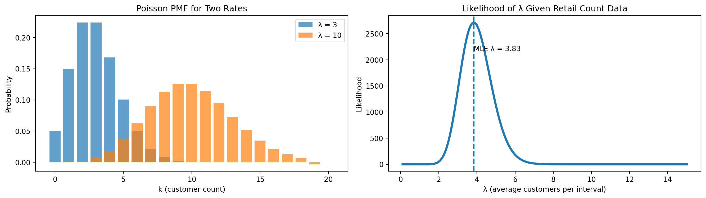
Visualization

• Left plot → PMF for \(\lambda = 3\) and \(\lambda = 10\)
  
• Right plot → likelihood as a function of \(\lambda\)

Bernoulli Distribution

The Bernoulli Distribution models the most fundamental probabilistic question in data analytics and business decision-making:

Two Possible Outcomes

Did an event happen or not?

A Bernoulli random variable has only two possible outcomes:

• success
  
• failure

These outcomes can be represented in multiple equivalent ways depending on context:

• yes / no
  
• 1 / 0
  
• click / no click
  
• purchase / no purchase
  
• tail / head (ղուշ / գիր)
  

Mathematical Definition

A random variable \(X\) follows a Bernoulli distribution if:

\[ X \sim \text{Bernoulli}(p) \]

where:

• \(p \in [0,1]\) is the probability of success

What Is a Bernoulli Trial

A Bernoulli trial is a single experiment with:

• exactly one attempt
• exactly two possible outcomes
• a fixed probability of success

Each trial is assumed to be independent.

Examples of Bernoulli Trials

Common real-world Bernoulli trials include:

• Did a user click an advertisement?
  
• Did a customer complete a purchase?
  
• Did a transaction fail?
  
• Did a device respond to a health check?

Each produces a binary outcome.

Real-World Narrative

Consider an online store tracking customer conversions.

For each user session:

• Purchase → 1
  
• No purchase → 0

Across thousands of sessions:

• Some users convert
  
• Most users do not

Each session is evaluated independently, with the same underlying probability of conversion.

Business Use Cases

Typical Bernoulli use cases in analytics:

• ad click behavior
  
• conversion events
  
• email engagement
  
• fraud detection flags
  
• churn indicators

Bernoulli is the building block for many advanced models.

Probability Mass Function (PMF)

Because Bernoulli is a discrete distribution, it is described by a Probability Mass Function (PMF):

\[ P(X = x) = p^x (1-p)^{1-x}, \quad x \in \{0,1\} \]

PMF Interpretation

This formula yields exactly two probabilities:

• \(P(X = 1) = p\)
  
• \(P(X = 0) = 1 - p\)

Expected Value and Variance

For a Bernoulli random variable:

\[ E[X] = p \]

\[ Var(X) = p(1-p) \]

Interpretation of Moments

• Expected value equals the probability of success
• Variance is largest at \(p = 0.5\)
• Variance shrinks as outcomes become more certain

• Large \(p\) → success likely
  
• Small \(p\) → success rare

Concrete Examples

• \(p = 0.02\) → 2% conversion rate
  
• \(p = 0.35\) → 35% email open rate
  
• \(p = 0.90\) → highly reliable system

Business Context

An e-commerce company records whether each visitor completes a purchase.

Each session is encoded as:

• 1 → purchase
  
• 0 → no purchase

Observed Data

{.smaller}

Session	Purchase
1	0
2	1
3	0
4	0
5	1
6	0
7	1
8	0
9	0
10	1

Summary Statistics

Let \(X\) be the purchase indicator per session.

• Number of sessions: \(n = 10\)
  
• Total purchases: \(S = 4\)

Sample mean:

\[ \bar{x} = \frac{4}{10} = 0.4 \]

Estimated probability:

\[ \hat{p} = 0.4 \]

Defining the Random Variable

\[ X = \begin{cases} 1 & \text{if a purchase occurs} \\ 0 & \text{otherwise} \end{cases} \]

A Bernoulli model is an appropriate first representation of this process.

So Far …

Final Intuition Summary

• Use Uniform for “random within limits.”
• Use Exponential for “time until next event.”
• Use Poisson for “number of events per interval.”
• Use Bernoulli for “one yes/no outcome”.

CLT

“Even if you’re not normal, the average is normal”

The Magic of the Normal Distribution

The Normal distribution appears everywhere in data.

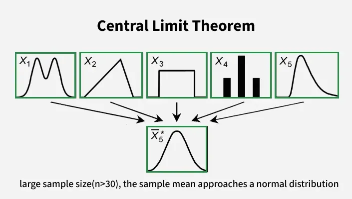
What the Central Limit Theorem Says

The Central Limit Theorem states:

• When we take the mean of many independent random variables
• regardless of the shape of the original distribution
• provided they have finite mean and variance
• the distribution of the sample mean becomes approximately Normal as the sample size grows

in other words…

.

Intuition Behind the CLT

• Real-world data often come from skewed or irregular distributions.
• But when we average many small effects, the result tends toward a bell shape.
• This “averaging effect” is why the Normal distribution is so common.

Why This Matters in Analytics

The CLT allows us to:

• build confidence intervals
• perform hypothesis tests
• use Normal-based statistical tools
• approximate distributions of sums and averages

Even when the original data are not Normal.

Non-Normal Data Example

Think about:

• waiting times (often skewed)
• revenue per customer (heavy-tailed)
• customer arrival counts (discrete)

Individually, these can be far from Normal.

When we repeatedly take many samples and compute means:

• the distribution of the means becomes more symmetric
• it approaches the characteristic bell curve
• this happens regardless of the original shape

Simulation: Visualizing CLT

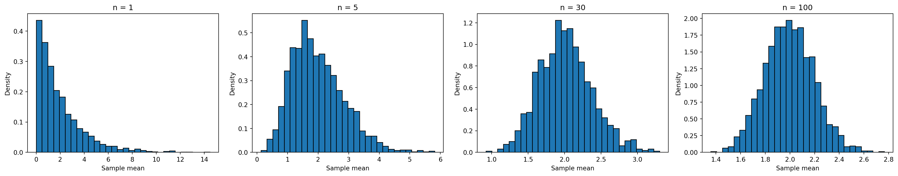
What the Simulation Shows

• For small n, the distribution of sample means is skewed.
• As n increases:
  • the distribution becomes more symmetric
  • it approaches a bell shape
  • even though the original data were not Normal

Conditions for CLT

Before applying CLT:

• samples should be independent
• sample size should be sufficiently large
• underlying distribution must have finite variance

These ensure the sample mean behaves approximately Normal.

Practical Rules of Thumb (heuristics in analytics)

• If original data are nearly Normal → small n is ok
  
• If data are skewed → larger n is needed
  
• n ≥ 30 often yields good Normal approximation

Applying CLT in Practice

• confidence interval construction
  
• hypothesis testing
  
• A/B testing rules
  
• regression inference

These methods assume approximate Normality of averages.

“Even if you’re not normal, the average is normal.”